02 - Dimension reduction and discretization

In this notebook, we will cover how to perform dimension reduction and discretization of molecular dynamics data. We also repeat data loading and visualization tasks from Notebook 01 ➜ 📓.

Maintainers: [@cwehmeyer](https://github.com/cwehmeyer), [@marscher](https://github.com/marscher), [@thempel](https://github.com/thempel), [@psolsson](https://github.com/psolsson)

Remember: - to run the currently highlighted cell, hold ⇧ Shift and press ⏎ Enter; - to get help for a specific function, place the cursor within the function’s brackets, hold ⇧ Shift, and press ⇥ Tab; - you can find the full documentation at PyEMMA.org.

%matplotlib inline
import matplotlib.pyplot as plt
import numpy as np
import mdshare
import pyemma

/storage/mi/marscher/software/miniconda3/conda-bld/pyemma-doc_1607519340854/_h_env_placehold_placehold_placehold_placehold_placehold_placehold_placehold_placehold_placehold_placehold_placehold_placehold_placehold_placehold_placehold_placehold_placehold_pl/lib/python3.9/site-packages/mdshare/repository.py:53: YAMLLoadWarning: calling yaml.load() without Loader=... is deprecated, as the default Loader is unsafe. Please read https://msg.pyyaml.org/load for full details.
  data = load(fh)

Case 1: preprocessed, two-dimensional data (toy model)

We load the two-dimensional trajectory from an archive using numpy (see Notebook 01 ➜ 📓) and visualize the marginal and joint distributions of both components. In order to make the important concept of metastability easier to understand, an excerpt from the original trajectory is added.

file = mdshare.fetch('hmm-doublewell-2d-100k.npz', working_directory='data')
with np.load(file) as fh:
    data = fh['trajectory']

fig, axes = plt.subplots(1, 2, figsize=(10, 4))
pyemma.plots.plot_feature_histograms(data, feature_labels=['$x$', '$y$'], ax=axes[0])
for i, dim in enumerate(['y', 'x']):
    axes[0].plot(data[:300, 1 - i], np.linspace(-0.2 + i, 0.8 + i, 300), color='C2', alpha=0.6)
    axes[0].annotate(
        '${}$(time)'.format(dim),
        xy=(3, 0.6 + i),
        xytext=(3, i),
        arrowprops=dict(fc='C2', ec='None', alpha=0.6, width=2))
pyemma.plots.plot_density(*data.T, ax=axes[1])
axes[1].set_xlabel('$x$')
axes[1].set_ylabel('$y$')
axes[1].set_xlim(-4, 4)
axes[1].set_ylim(-4, 4)
axes[1].set_aspect('equal')
fig.tight_layout()

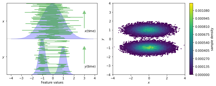
Given the low dimensionality of this data set, we can directly attempt to discretize, e.g., with \(k\)-means with \(100\) centers and a stride of \(5\) to reduce the computational effort. In real world examples we also might encounter low dimensional feature spaces which do not require further dimension reduction techniques to be clustered efficiently.

cluster_kmeans = pyemma.coordinates.cluster_kmeans(data, k=100, stride=5)

09-12-20 14:23:04 pyemma.coordinates.clustering.kmeans.KmeansClustering[0] WARNING  Algorithm did not reach convergence criterion of 1e-05 in 10 iterations. Consider increasing max_iter.

WARNING:pyemma.coordinates.clustering.kmeans.KmeansClustering[0]:Algorithm did not reach convergence criterion of 1e-05 in 10 iterations. Consider increasing max_iter.

… or with a regspace technique where all centers should have a minimal pairwise distance of \(0.5\) units of length.

cluster_regspace = pyemma.coordinates.cluster_regspace(data, dmin=0.5)

We visualize both sets of centers on top of the joint distribution:

fig, axes = plt.subplots(1, 2, figsize=(10, 4))
for ax, cls in zip(axes.flat, [cluster_kmeans, cluster_regspace]):
    pyemma.plots.plot_density(*data.T, ax=ax, cbar=False, alpha=0.1)
    ax.scatter(*cls.clustercenters.T, s=15, c='C1')
    ax.set_xlabel('$x$')
    ax.set_xlim(-4, 4)
    ax.set_ylim(-4, 4)
    ax.set_aspect('equal')
axes[0].set_ylabel('$y$')
fig.tight_layout()

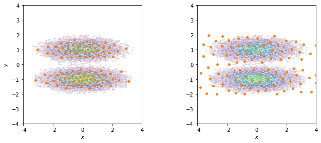
Have you noticed how the \(k\)-means centers follow the density of the data points while the regspace centers are spread uniformly over the whole area?

If your are only interested in well sampled states, you should use a density based method to discretize. If exploring new states is one of your objectives, it might be of advantage to place states also in rarely observed regions. The latter is especially useful in adaptive sampling approaches, because in the initial phase you want to explore the phase space as much as possible. The downside of placing states in areas of low density is that we will have poor statistics on these states.

Another advantage of regular space clustering is that it is fast in comparison to \(k\)-means: regspace clustering runs in linear time while \(k\)-means is superpolynomial in time.

⚠️ For large datasets we also offer a mini batch version of \(k\)-means which has the same semantics as the original method but trains the centers on subsets of your data. This tutorial does not cover this case, but you should keep in mind that \(k\)-means requires your low dimensional space to fit into your main memory.

As the number of cluster centers has to be chosen by the modeler, we will analyze its implications on the MSM analysis in Notebook 03 ➜ 📓. A systematic approach to choose this number is proposed in Notebook 00 ➜ 📓.

The main result of a discretization for Markov modeling, however, is not the set of centers but the time series of discrete states. These are accessible via the dtrajs attribute of any clustering object:

print(cluster_kmeans.dtrajs)
print(cluster_regspace.dtrajs)

[array([76, 62, 55, ..., 28, 53, 57], dtype=int32)]
[array([ 0,  1, 40, ..., 49, 14,  9], dtype=int32)]

For each trajectory passed to the clustering object, we get a corresponding discrete trajectory.

Please note that as an alternative to clustering algorithms such as \(k\)-means and regspace, it is possible to manually assign the data to cluster centers using the pyemma.coordinates.assign_to_centers() function.

Instead of discretizing the full (two-dimensional) space, we can attempt to find a one-dimensional subspace which 1. describes the slow dynamics of the data set equally well but 2. is easier to discretize.

One widespread method for dimension reduction is the principal component analysis (PCA) which finds a subspace with maximized variance:

pca = pyemma.coordinates.pca(data, dim=1)
pca_output = pca.get_output()
print(pca_output)

[array([[-0.26751208],
       [ 0.37113857],
       [-0.35730326],
       ...,
       [-0.55788803],
       [ 0.9381754 ],
       [-0.73651516]], dtype=float32)]

Another technique is the time-lagged independent component analysis (TICA) which finds a subspace with maximized autocorrelation molgedey-94, perez-hernandez-13. To compute the autocorrelation, we need a time shifted version of the data. This time shift is specified by the lag argument. For the current example, we choose a lag time of \(1\) step.

tica = pyemma.coordinates.tica(data, dim=1, lag=1)
tica_output = tica.get_output()
print(tica_output)

[array([[-0.42423657],
       [-0.73914737],
       [-0.79901934],
       ...,
       [-1.1870486 ],
       [-0.6090164 ],
       [-0.5659988 ]], dtype=float32)]

Instead of TICA, we can also employ the variational approach for Markov processes (VAMP) to obtain a coordinate transform wu-17. In contrast to TICA, VAMP can be applied to non-equilibrium / non-reversible data.

vamp = pyemma.coordinates.vamp(data, dim=1, lag=1)
vamp_output = vamp.get_output()
print(vamp_output)

[array([[0.5199959 ],
       [0.9068548 ],
       [0.97952616],
       ...,
       [1.4551867 ],
       [0.7478528 ],
       [0.6933637 ]], dtype=float32)]

⚠️ While there are many cases where PCA can find a suitable subspace, there are also many cases where the PCA-based subspace neglects the slow dynamics.

In our example, the slow process is the jump between both wells along the \(y\)-axis while the \(x\)-axis contains only random noise. For all three methods, we show the distribution after projecting the full dynamics onto a one-dimensional subspace (left) and the direction of projection (right).

pca_concatenated = pca_output[0]
tica_concatenated = tica_output[0]
vamp_concatenated = vamp_output[0]

fig, axes = plt.subplots(1, 2, figsize=(10, 4))
pyemma.plots.plot_feature_histograms(
    np.concatenate([pca_concatenated, tica_concatenated, vamp_concatenated], axis=1),
    feature_labels=['PCA', 'TICA', 'VAMP'],
    ax=axes[0])
pyemma.plots.plot_density(*data.T, ax=axes[1], cbar=False, alpha=0.1)
axes[1].plot(
    [0, 3 * pca.eigenvectors[0, 0]],
    [0, 3 * pca.eigenvectors[1, 0]],
    linewidth=3,
    label='PCA')
axes[1].plot(
    [0, 3 * tica.eigenvectors[0, 0]],
    [0, 3 * tica.eigenvectors[1, 0]],
    linewidth=3,
    label='TICA')
axes[1].plot(
    [0, 3 * vamp.singular_vectors_right[0, 0]],
    [0, 3 * vamp.singular_vectors_right[1, 0]],
    linewidth=3,
    label='VAMP')
axes[1].set_xlabel('$x$')
axes[1].set_ylabel('$y$')
axes[1].set_xlim(-4, 4)
axes[1].set_ylim(-4, 4)
axes[1].set_aspect('equal')
axes[1].legend()
fig.tight_layout()

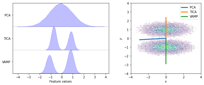
We see that TICA and VAMP project along the \(y\)-axis and, thus, yield a subspace which clearly resolves both metastable states. PCA on the other hand projects closely along the \(x\)-axis and does not resolve both metastable states. This is a case in point where variance maximization does not find a subspace which resolves the relevant dynamics of the system.

This effect can also be seen when we plot the subspace time series:

fig, ax = plt.subplots(figsize=(10, 3))
ax.plot(pca_concatenated[:300], label='PCA')
ax.plot(tica_concatenated[:300], label='TICA')
# note that for better comparability, we enforce the same direction as TICA
ax.plot(vamp_concatenated[:300] * -1, label='VAMP')
ax.set_xlabel('time / steps')
ax.set_ylabel('feature values')
ax.legend()
fig.tight_layout()

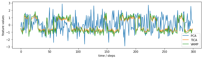
In case of TICA/VAMP, we observe that the projected coordinate jumps between two clearly separated plateaus. For PCA, we observe only random fluctuations without any hint of metastablility.

In many applications, however, we also need to understand what our coordinate transform means in physical terms. This, in general, might be less obvious. Hence, it might be instructive to inspect the correlations of features to the independent components:

fig, ax = plt.subplots()
i = ax.imshow(tica.feature_TIC_correlation, cmap='bwr', vmin=-1, vmax=1)

ax.set_xticks([0])
ax.set_xlabel('IC')

ax.set_yticks([0, 1])
ax.set_ylabel('input feature')

fig.colorbar(i);

<matplotlib.colorbar.Colorbar at 0x7f6a2e380e50>

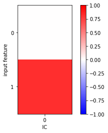
In this simple example, we clearly see a significant correlation between the \(y\) component of the input data and the first independent component.

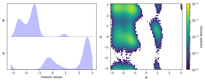
Case 2: low-dimensional molecular dynamics data (alanine dipeptide)

We fetch the alanine dipeptide data set, load the backbone torsions into memory, and visualize the margial and joint distributions:

pdb = mdshare.fetch('alanine-dipeptide-nowater.pdb', working_directory='data')
files = mdshare.fetch('alanine-dipeptide-*-250ns-nowater.xtc', working_directory='data')

feat = pyemma.coordinates.featurizer(pdb)
feat.add_backbone_torsions(periodic=False)
data = pyemma.coordinates.load(files, features=feat)
data_concatenated = np.concatenate(data)

fig, axes = plt.subplots(1, 2, figsize=(10, 4))
pyemma.plots.plot_feature_histograms(
    np.concatenate(data), feature_labels=['$\Phi$', '$\Psi$'], ax=axes[0])
pyemma.plots.plot_density(*data_concatenated.T, ax=axes[1], logscale=True)
axes[1].set_xlabel('$\Phi$')
axes[1].set_ylabel('$\Psi$')
fig.tight_layout()

Following the previous example, we perform a \(k\)-means (\(100\) centers, stride of \(5\)) and a regspace clustering (\(0.3\) radians center distance) on the full two-dimensional data set and visualize the obtained centers. In Notebook 03 ➜ 📓, we show the effect of different numbers of cluster centers on MSM estimation.

cluster_kmeans = pyemma.coordinates.cluster_kmeans(data, k=100, max_iter=50, stride=5)
cluster_regspace = pyemma.coordinates.cluster_regspace(data, dmin=0.3)

fig, axes = plt.subplots(1, 2, figsize=(10, 4), sharex=True, sharey=True)
for ax, cls in zip(axes.flat, [cluster_kmeans, cluster_regspace]):
    pyemma.plots.plot_density(*data_concatenated.T, ax=ax, cbar=False, alpha=0.1, logscale=True)
    ax.scatter(*cls.clustercenters.T, s=15, c='C1')
    ax.set_xlabel('$\Phi$')
    ax.set_ylabel('$\Psi$')
fig.tight_layout()

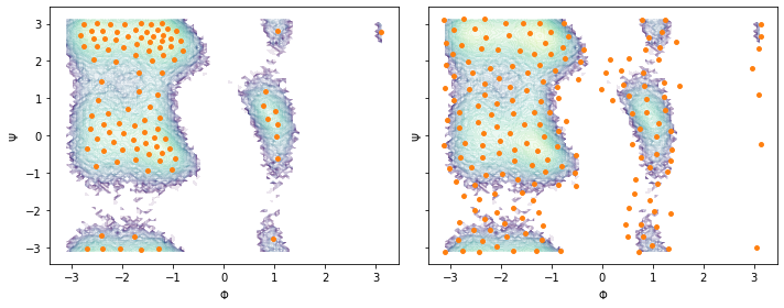
Again, notice the difference between \(k\)-means and regspace clustering.

Now, we use a different featurization for the same data set and revisit how to use PCA, TICA, and VAMP.

⚠️ In practice you almost never would like to use PCA as dimension reduction method in MSM building, as it does not preserve kinetic variance. We are showing it here in these exercises to make this point clear.

Streaming memory discretization

For real world case examples it is often not possible to load entire datasets into main memory. We can perform the whole discretization step without the need of having the dataset fit into memory. Keep in mind that this is not as efficient as loading into memory, because certain calculations (e.g. featurization), will have to be recomputed during iterations.

reader = pyemma.coordinates.source(files, top=pdb) # create reader
reader.featurizer.add_backbone_torsions(periodic=False) # add feature
tica = pyemma.coordinates.tica(reader) # perform tica on feature space
cluster = pyemma.coordinates.cluster_mini_batch_kmeans(tica, k=10, batch_size=0.1, max_iter=3) # cluster in tica space
# get result
dtrajs = cluster.dtrajs
print('discrete trajectories:', dtrajs)

09-12-20 14:27:31 pyemma.coordinates.clustering.kmeans.MiniBatchKmeansClustering[20] INFO     Algorithm did not reach convergence criterion of 1e-05 in 3 iterations. Consider increasing max_iter.

INFO:pyemma.coordinates.clustering.kmeans.MiniBatchKmeansClustering[20]:Algorithm did not reach convergence criterion of 1e-05 in 3 iterations. Consider increasing max_iter.

discrete trajectories: [array([9, 9, 9, ..., 2, 6, 6], dtype=int32), array([9, 9, 9, ..., 7, 7, 7], dtype=int32), array([9, 2, 1, ..., 7, 7, 7], dtype=int32)]

We should mention that regular space clustering does not require to load the TICA output into memory, while \(k\)-means does. Use the minibatch version if your TICA output does not fit memory. Since the minibatch version takes more time to converge, it is therefore desirable to to shrink the TICA output to fit into memory. We split the pipeline for cluster estimation, and re-use the reader to for the assignment of the full dataset.

cluster = pyemma.coordinates.cluster_kmeans(tica, k=10, stride=3) # use only 1/3 of the input data to find centers

09-12-20 14:28:34 pyemma.coordinates.clustering.kmeans.KmeansClustering[21] WARNING  Algorithm did not reach convergence criterion of 1e-05 in 10 iterations. Consider increasing max_iter.

WARNING:pyemma.coordinates.clustering.kmeans.KmeansClustering[21]:Algorithm did not reach convergence criterion of 1e-05 in 10 iterations. Consider increasing max_iter.

Have you noticed how fast this converged compared to the minibatch version? We can now just obtain the discrete trajectories by accessing the property on the cluster instance. This will get all the TICA projected trajectories and assign them to the centers computed on the reduced data set.

dtrajs = cluster.dtrajs
print('Assignment:', dtrajs)
dtrajs_len = [len(d) for d in dtrajs]
for dtraj_len, input_len in zip(dtrajs_len, reader.trajectory_lengths()):
    print('Input length:', input_len, '\tdtraj length:', dtraj_len)

Assignment: [array([4, 4, 4, ..., 4, 1, 1], dtype=int32), array([4, 4, 4, ..., 8, 0, 8], dtype=int32), array([4, 9, 7, ..., 0, 0, 8], dtype=int32)]
Input length: 250000    dtraj length: 250000
Input length: 250000    dtraj length: 250000
Input length: 250000    dtraj length: 250000

Exercise 1: data loading

Load the heavy atoms’ positions into memory.

Solution

feat = pyemma.coordinates.featurizer(pdb)
feat.add_selection(feat.select_Heavy())
data = pyemma.coordinates.load(files, features=feat)

print('We have {} features.'.format(feat.dimension()))

fig, ax = plt.subplots(figsize=(10, 7))
pyemma.plots.plot_feature_histograms(np.concatenate(data), feature_labels=feat, ax=ax)
fig.tight_layout()

We have 30 features.

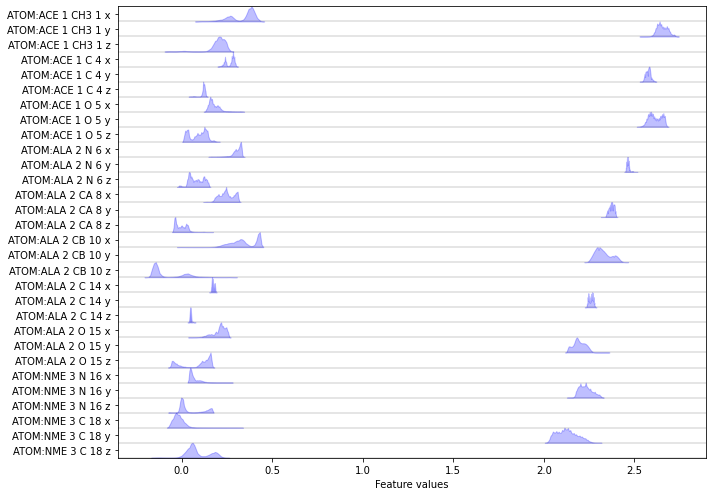
Discretizing a \(30\)-dimensional feature space is impractical. Let’s use PCA to find a low-dimensional projection and visualize the marginal distributions of all principal components (PCs) as well as the joint distributions for the first two PCs:

pca = pyemma.coordinates.pca(data)
pca_concatenated = np.concatenate(pca.get_output())

fig, axes = plt.subplots(1, 3, figsize=(12, 3), sharex=True)
pyemma.plots.plot_feature_histograms(
    pca_concatenated, ['PC {}'.format(i + 1) for i in range(pca.dimension())], ax=axes[0])
pyemma.plots.plot_density(*pca_concatenated[:, :2].T, ax=axes[1], cbar=False, logscale=True)
pyemma.plots.plot_free_energy(*pca_concatenated[:, :2].T, ax=axes[2], legacy=False)
for ax in axes.flat[1:]:
    ax.set_xlabel('PC 1')
    ax.set_ylabel('PC 2')
fig.tight_layout()

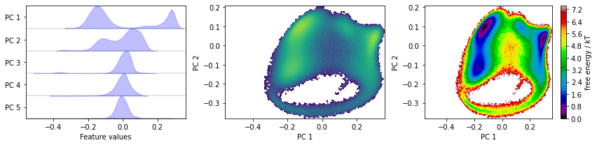
With the default parameters, PCA will return as many dimensions as necessary to explain \(95\%\) of the variance; in this case, we have found a five-dimensional subspace which does seem to resolve some metastability in the first three principal components.

Exercise 2: TICA visualization

Apply TICA and visualize the marginal distributions of all independent components (ICs) as well as the joint distributions of the first two ICs.

Solution

tica = pyemma.coordinates.tica(data)
tica_concatenated = np.concatenate(tica.get_output())

fig, axes = plt.subplots(1, 3, figsize=(12, 3))
pyemma.plots.plot_feature_histograms(
    tica_concatenated, ['IC {}'.format(i + 1) for i in range(tica.dimension())], ax=axes[0])
pyemma.plots.plot_density(*tica_concatenated[:, :2].T, ax=axes[1], cbar=False, logscale=True)
pyemma.plots.plot_free_energy(*tica_concatenated[:, :2].T, ax=axes[2], legacy=False)
for ax in axes.flat[1:]:
    ax.set_xlabel('IC 1')
    ax.set_ylabel('IC 2')
fig.tight_layout()

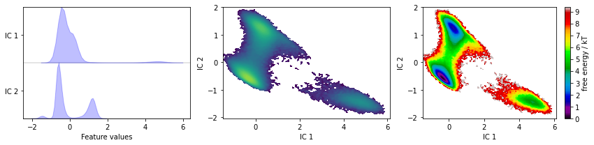
TICA, by default, uses a lag time of \(10\) steps, kinetic mapping and a kinetic variance cutoff of \(95\%\) to determine the number of ICs. We observe that this projection does resolve some metastability in both ICs. Whether these projections are suitable for building Markov state models, though, remains to be seen in later tests (Notebook 03 ➜ 📓).

As we discussed in the first example, the physical meaning of the TICA projection is not directly clear. We can analyze the feature TIC correlation as we did above:

fig, ax = plt.subplots(figsize=(3, 8))
i = ax.imshow(tica.feature_TIC_correlation, cmap='bwr')

ax.set_xticks(range(tica.dimension()))
ax.set_xlabel('IC')

ax.set_yticks(range(feat.dimension()))
ax.set_yticklabels(feat.describe())
ax.set_ylabel('input feature')

fig.colorbar(i);

<matplotlib.colorbar.Colorbar at 0x7f6a40254250>

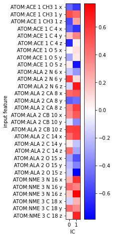
This is not helpful as it only shows that some of our \(x, y, z\)-coordinates correlate with the TICA components. Since we rather expect the slow processes to happen in backbone torsion space, this comes to no surprise.

To understand what the TICs really mean, let us do a more systematic approach and scan through some angular features. We add some randomly chosen angles between heavy atoms and the backbone angles that we already know to be a good feature:

feat_test = pyemma.coordinates.featurizer(pdb)
feat_test.add_backbone_torsions(periodic=False)
feat_test.add_angles(feat_test.select_Heavy()[:-1].reshape(3, 3), periodic=False)
data_test = pyemma.coordinates.load(files, features=feat_test)
data_test_concatenated = np.concatenate(data_test)

For the sake of simplicity, we use scipy’s implementation of Pearson’s correlation coefficient which we compute between our test features and TICA projected \(x, y, z\)-coordinates:

from scipy.stats import pearsonr
test_feature_TIC_correlation = np.zeros((feat_test.dimension(), tica.dimension()))

for i in range(feat_test.dimension()):
    for j in range(tica.dimension()):
        test_feature_TIC_correlation[i, j] = pearsonr(
            data_test_concatenated[:, i],
            tica_concatenated[:, j])[0]

vm = abs(test_feature_TIC_correlation).max()

fig, ax = plt.subplots()
i = ax.imshow(test_feature_TIC_correlation, vmin=-vm, vmax=vm, cmap='bwr')

ax.set_xticks(range(tica.dimension()))
ax.set_xlabel('IC')

ax.set_yticks(range(feat_test.dimension()))
ax.set_yticklabels(feat_test.describe())
ax.set_ylabel('input feature')

fig.colorbar(i);

<matplotlib.colorbar.Colorbar at 0x7f6a2d3c59a0>

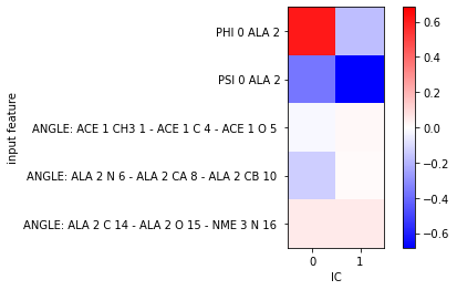
From this simple analysis, we find that features that correlated most with our TICA projection are indeed the backbone torsion angles used previously. We might thus expect the dynamics in TICA space to be similar to the one in backbone torsion space.

⚠️ Please note that in general, we do not know which feature would be a good observable. Thus, a realistic scenario might require a much broader scan of a large set of different features.

However, it should be mentioned that TICA projections do not necessarily have a simple physical interpretation. The above analysis might very well end with feature TIC correlations that show no significant contributor and rather hint towards a complicated linear combination of input features.

As an alternative to understanding the projection in detail at this stage, one might go one step further and extract representative structures, e.g., from an MSM, as shown in Notebook 05 📓.

Exercise 3: PCA parameters

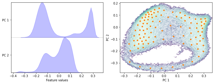
Perform PCA on the heavy atoms’ positions data set with a target dimension of two; then discretize the two-dimensional subspace using \(k\)-means with \(100\) centers and a stride of \(5\) to reduce the computational effort.

Hint: Look up the parameters of pyemma.coordinates.pca(), especially the dim parameter.

Solution

pca = pyemma.coordinates.pca(data, dim=2)
pca_concatenated = np.concatenate(pca.get_output())

cluster = pyemma.coordinates.cluster_kmeans(pca, k=100, max_iter=50, stride=5)

fig, axes = plt.subplots(1, 2, figsize=(10, 4))
pyemma.plots.plot_feature_histograms(
    pca_concatenated, ['PC {}'.format(i + 1) for i in range(pca.dimension())], ax=axes[0])
pyemma.plots.plot_density(*pca_concatenated.T, ax=axes[1], cbar=False, alpha=0.1, logscale=True)
axes[1].scatter(*cluster.clustercenters.T, s=15, c='C1')
axes[1].set_xlabel('PC 1')
axes[1].set_ylabel('PC 2')
fig.tight_layout()

Exercise 4: TICA parameters

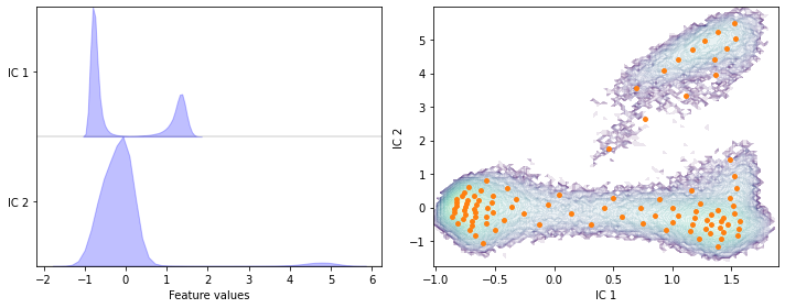
Perform TICA at lag time \(1\) step on the heavy atoms’ positions data set with a target dimension of two; then discretize the two-dimensional subspace using \(k\)-means with \(100\) centers and a stride of \(5\) to reduce the computational effort.

Hint: Look up the parameters of pyemma.coordinates.tica(), especially the dim and lag parameters.

Solution

tica = pyemma.coordinates.tica(data, lag=1, dim=2)
tica_concatenated = np.concatenate(tica.get_output())

cluster = pyemma.coordinates.cluster_kmeans(tica, k=100, max_iter=50, stride=5)

fig, axes = plt.subplots(1, 2, figsize=(10, 4))
pyemma.plots.plot_feature_histograms(
    tica_concatenated, ['IC {}'.format(i + 1) for i in range(tica.dimension())], ax=axes[0])
pyemma.plots.plot_density(*tica_concatenated.T, ax=axes[1], cbar=False, alpha=0.1, logscale=True)
axes[1].scatter(*cluster.clustercenters.T, s=15, c='C1')
axes[1].set_xlabel('IC 1')
axes[1].set_ylabel('IC 2')
fig.tight_layout()

Have you noticed the difference in the first two ICs for lag times \(10\) steps vs. \(1\) step (e.g., result of exercises \(2\) and \(3\))?

Case 3: another molecular dynamics data set (pentapeptide)

Before we start to load and discretize the pentapeptide data set, let us discuss what the difficulties with larger protein systems are. The goal of this notebook is to find a state space discretization for MSM estimation. This means that an algorithm such as \(k\)-means has to be able to find a meaningful state space partitioning. In general, this works better in lower dimensional spaces because Euclidean distances become less meaningful with increasing dimensionality aggarwal-01. The modeler should be aware that a discretization of hundreds of dimensions will be computationally expensive and most likely yield unsatisfactory results.

The first goal is thus to map the data to a reasonable number of dimensions, e.g., with a smart choice of features and/or by using TICA. Large systems often require significant parts of the kinetic variance to be discarded in order to obtain a balance between capturing as much of the kinetic variance as possible and achieving a reasonable discretization.

Another point about discretization algorithms is that one should bear in mind the distribution of density. The \(k\)-means algorithm tends to conserve density, i.e., data sets that incorporate regions of extremely high density as well as poorly sampled regions might be problematic, especially in high dimensions. For those cases, a regular spatial clustering might be worth a try.

More details on problematic data situations and how to cope with them are explained in Notebook 08 📓.

Now, we fetch the pentapeptide data set, load several different input features into memory and perform a VAMP estimation/scoring of each. Since we want to evaluate the VAMP score on a disjoint test set, we split the available files into a train and test set.

pdb = mdshare.fetch('pentapeptide-impl-solv.pdb', working_directory='data')
files = mdshare.fetch('pentapeptide-*-500ns-impl-solv.xtc', working_directory='data')

feat = pyemma.coordinates.featurizer(pdb)
feat.add_backbone_torsions(cossin=True, periodic=False)
feat.add_sidechain_torsions(which='all', cossin=True, periodic=False)

train_files = files[:-2]
test_file = files[-2]  # last trajectory is our test data set
assert set(train_files) & set(test_file) == set()  # ensure test and train sets do not overlap

data_torsions = pyemma.coordinates.load(train_files, features=feat)
data_torsions_test = pyemma.coordinates.load(test_file, features=feat)

feat.active_features = []
feat.add_distances_ca(periodic=False)

data_dists_ca = pyemma.coordinates.load(train_files, features=feat)
data_dists_ca_test = pyemma.coordinates.load(test_file, features=feat)

feat.active_features = []
pairs = feat.pairs(feat.select_Heavy())
feat.add_contacts(pairs, periodic=False)

data_contacts = pyemma.coordinates.load(train_files, features=feat)
data_contacts_test = pyemma.coordinates.load(test_file, features=feat)

/storage/mi/marscher/software/miniconda3/conda-bld/pyemma-doc_1607519340854/_h_env_placehold_placehold_placehold_placehold_placehold_placehold_placehold_placehold_placehold_placehold_placehold_placehold_placehold_placehold_placehold_placehold_placehold_pl/lib/python3.9/site-packages/mdtraj/geometry/dihedral.py:374: FutureWarning: arrays to stack must be passed as a "sequence" type such as list or tuple. Support for non-sequence iterables such as generators is deprecated as of NumPy 1.16 and will raise an error in the future.
  indices = np.vstack(x for x in indices if x.size)[id_sort]
/storage/mi/marscher/software/miniconda3/conda-bld/pyemma-doc_1607519340854/_h_env_placehold_placehold_placehold_placehold_placehold_placehold_placehold_placehold_placehold_placehold_placehold_placehold_placehold_placehold_placehold_placehold_placehold_pl/lib/python3.9/site-packages/pyemma/coordinates/data/featurization/angles.py:211: FutureWarning: arrays to stack must be passed as a "sequence" type such as list or tuple. Support for non-sequence iterables such as generators is deprecated as of NumPy 1.16 and will raise an error in the future.
  indices = np.vstack(valid.values())

def plot_for_lag(ax, lag, dim=3):
    vamp_torsions = pyemma.coordinates.vamp(data_torsions, lag=lag, dim=dim)
    vamp_dist_ca = pyemma.coordinates.vamp(data_dists_ca, lag=lag, dim=dim)
    vamp_contacts = pyemma.coordinates.vamp(data_contacts, lag=lag, dim=dim)

    vamps = (vamp_torsions, vamp_dist_ca, vamp_contacts)
    test_data = (data_torsions_test, data_dists_ca_test, data_contacts_test)
    labels = ('torsions', 'CA distances', 'contacts')
    for i, (v, test_data) in enumerate(zip(vamps, test_data)):
        s = v.score(test_data=test_data)
        ax.bar(i, s)
    ax.set_title('VAMP2 @ lag = {} ps'.format(lag))
    ax.set_xticks(range(len(vamps)))
    ax.set_xticklabels(labels)
    fig.tight_layout()

fig, axes = plt.subplots(1, 4, figsize=(15, 3), sharey=True)
plot_for_lag(axes[0], 5)
plot_for_lag(axes[1], 10)
plot_for_lag(axes[2], 20)
plot_for_lag(axes[3], 50)

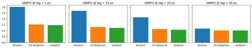
For the small lag time we see that there is a large gap between torsion angles on the one hand and CA distances and contacts on the other hand. For increasing lag times this gap vanishes, but also the overall score is decreasing. Because we have capped the maximum dimension or equivalently the score to contain only the three largest components of the underlying dynamical model, we can expect only a maximum score of three. As we increase the lag time, more of the fast kinetic processes have already decayed. So these are not contributing to the score anymore.

We have learned that backbone and sidechain torsions are better suited than the other features for modeling the kinetics, so we will continue with this feature.

data_concatenated = data_torsions + [data_torsions_test] # concatenate two lists
type(data_concatenated)

list

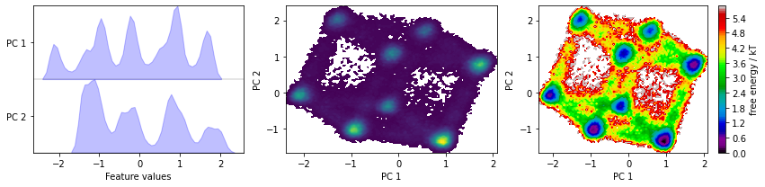
We now perform a principal component analysis (PCA) with default parameters and visualize the marginal distributions of all PCs and the joint distributions of the first two PCs.

pca = pyemma.coordinates.pca(data_concatenated, dim=2)
pca_concatenated = np.concatenate(pca.get_output())

fig, axes = plt.subplots(1, 3, figsize=(12, 3))
pyemma.plots.plot_feature_histograms(
    pca_concatenated,
    ['PC {}'.format(i + 1) for i in range(pca.dimension())],
    ax=axes[0])
pyemma.plots.plot_density(*pca_concatenated[:, :2].T, ax=axes[1], cbar=False)
pyemma.plots.plot_free_energy(*pca_concatenated[:, :2].T, ax=axes[2], legacy=False)
for ax in axes.flat[1:]:
    ax.set_xlabel('PC 1')
    ax.set_ylabel('PC 2')
fig.tight_layout()

We have a look at some TICA projections estimated with the lag times given below and, for each lag time, we visualize the marginal distributions of all ICs and the joint distributions of the first two ICs. The actual dimension is determined by the default variance cutoff of \(95\%\). This could be customized either by adjusting the var_cutoff or by requesting a certain number of dimensions with the dim keyword argument of tica().

lags = [1, 2, 5, 10, 20, 50]

fig, axes = plt.subplots(6, 3, figsize=(10, 18))
for i, lag in enumerate(lags):
    tica = pyemma.coordinates.tica(data_concatenated, lag=lag)
    tica_concatenated = np.concatenate(tica.get_output())
    pyemma.plots.plot_feature_histograms(
        tica_concatenated,
        ['IC {}'.format(i + 1) for i in range(tica.dimension())],
        ax=axes[i, 0])
    axes[i, 0].set_title('lag time = {} steps'.format(lag))
    axes[i, 1].set_title(
        'Density, actual dimension = {}'.format(tica.dimension()))
    pyemma.plots.plot_density(
        *tica_concatenated[:, :2].T, ax=axes[i, 1], cbar=False)
    pyemma.plots.plot_free_energy(
        *tica_concatenated[:, :2].T, ax=axes[i, 2], legacy=False)
for ax in axes[:, 1:].flat:
    ax.set_xlabel('IC 1')
    ax.set_ylabel('IC 2')
axes[0, 2].set_title('Pseudo free energy')
fig.tight_layout()

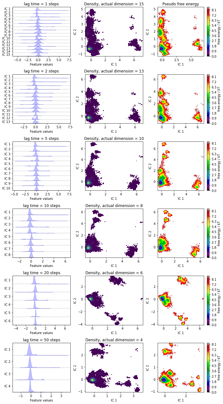
Have you noticed that increasing the lag time 1. leads to a rotation of the projection and 2. reduces the number of TICs to explain \(95\%\) (default) of the kinetic variance?

Note that, while we can get lower and lower dimensional subspaces with increased lag times, we also loose information from the faster processes.

How to choose the optimal lag time for a TICA projection often is a hard problem and there are only heuristic approaches to it. For example, you can search for the amount of dimensions where the variance cutoff does not change anymore.

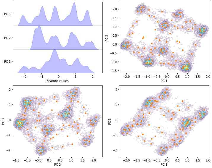
Perform PCA with target dimension \(3\) on the current feature set and discretize the projected space using \(k\)-means with \(100\) centers and a stride of \(5\) to reduce the computational effort.

Solution

pca = pyemma.coordinates.pca(data_concatenated, dim=3)
pca_concatenated = np.concatenate(pca.get_output(stride=5))

cluster = pyemma.coordinates.cluster_kmeans(pca, k=100, max_iter=50, stride=5)

fig, axes = plt.subplots(2, 2, figsize=(10, 8))
pyemma.plots.plot_feature_histograms(
    pca_concatenated, ['PC {}'.format(i + 1) for i in range(pca.dimension())], ax=axes[0, 0])
for ax, (i, j) in zip(axes.flat[1:], [[0, 1], [1, 2], [0, 2]]):
    pyemma.plots.plot_density(*pca_concatenated[:, [i, j]].T, ax=ax, cbar=False, alpha=0.1)
    ax.scatter(*cluster.clustercenters[:, [i, j]].T, s=15, c='C1')
    ax.set_xlabel('PC {}'.format(i + 1))
    ax.set_ylabel('PC {}'.format(j + 1))
fig.tight_layout()

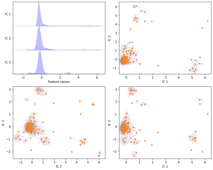
Perform TICA with target dimension \(3\) and lag time \(20\) steps on the current feature set and discretize the projected space using \(k\)-means with \(100\) centers and a stride of \(5\) to reduce the computational effort.

Solution

tica = pyemma.coordinates.tica(data_concatenated, dim=3)
tica_concatenated = np.concatenate(tica.get_output(stride=5))

cluster = pyemma.coordinates.cluster_kmeans(tica, k=100, max_iter=50, stride=5)

fig, axes = plt.subplots(2, 2, figsize=(10, 8))
pyemma.plots.plot_feature_histograms(
    tica_concatenated, ['IC {}'.format(i + 1) for i in range(tica.dimension())], ax=axes[0, 0])
for ax, (i, j) in zip(axes.flat[1:], [[0, 1], [1, 2], [0, 2]]):
    pyemma.plots.plot_density(
        *tica_concatenated[:, [i, j]].T, ax=ax, cbar=False, alpha=0.1)
    ax.scatter(*cluster.clustercenters[:, [i, j]].T, s=15, c='C1')
    ax.set_xlabel('IC {}'.format(i + 1))
    ax.set_ylabel('IC {}'.format(j + 1))
fig.tight_layout()

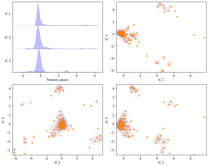
Perform VAMP with target dimension \(3\) and lag time \(20\) steps on the current feature set and discretize the projected space using \(k\)-means with \(100\) centers and a stride of \(5\) to reduce the computational effort.

Solution

vamp = pyemma.coordinates.vamp(data_concatenated, lag=20, dim=3)
vamp_concatenated = np.concatenate(vamp.get_output(stride=5))

cluster = pyemma.coordinates.cluster_kmeans(vamp, k=100, max_iter=50, stride=5)

fig, axes = plt.subplots(2, 2, figsize=(10, 8))
pyemma.plots.plot_feature_histograms(
    tica_concatenated, ['IC {}'.format(i + 1) for i in range(tica.dimension())], ax=axes[0, 0])
for ax, (i, j) in zip(axes.flat[1:], [[0, 1], [1, 2], [0, 2]]):
    pyemma.plots.plot_density(*vamp_concatenated[:, [i, j]].T, ax=ax, cbar=False, alpha=0.1)
    ax.scatter(*cluster.clustercenters[:, [i, j]].T, s=15, c='C1')
    ax.set_xlabel('IC {}'.format(i + 1))
    ax.set_ylabel('IC {}'.format(j + 1))
fig.tight_layout()

Wrapping up

In this notebook, we have learned how to reduce the dimension of molecular simulation data and discretize the projected dynamics with PyEMMA. In detail, we have used - pyemma.coordinates.pca() to perform a principal components analysis, - pyemma.coordinates.tica() to perform a time-lagged independent component analysis, and - pyemma.coordinates.vamp() to analyze the quality of some feature spaces, perform dimension reduction, and - pyemma.coordinates.cluster_kmeans() to perform a \(k\)-means clustering, and - pyemma.coordinates.cluster_regspace() to perform a regspace clustering.

References

[^]Molgedey, L. and Schuster, H. G.. 1994. Separation of a mixture of independent signals using time delayed correlations. URL

[^]Guillermo Pérez-Hernández and Fabian Paul and Toni Giorgino and Gianni De Fabritiis and Frank Noé. 2013. Identification of slow molecular order parameters for Markov model construction. URL

[^]Wu, H. and Noé, F.. 2017. Variational approach for learning Markov processes from time series data. URL

[^]Aggarwal, Charu C. and Hinneburg, Alexander and Keim, Daniel A.. 2001. On the Surprising Behavior of Distance Metrics in High Dimensional Space.