01 - Data-I/O and featurization

In this notebook, we will cover how to load (and visualize) data with PyEMMA. We are going to extract different features (collective variables) and compare how well these are suited for Markov state model building. Further, we will introduce the concept of streaming data, which is mandatory to work with large data sets.

As with the other notebooks, we employ multiple examples. The idea is, first, to highlight the fundamental ideas with a non-physical test system (diffusion in a 2D double-well potential) and, second, to demonstrate real-world applications with molecular dynamics data.

Maintainers: [@cwehmeyer](https://github.com/cwehmeyer), [@marscher](https://github.com/marscher), [@thempel](https://github.com/thempel), [@psolsson](https://github.com/psolsson)

Remember: - to run the currently highlighted cell, hold ⇧ Shift and press ⏎ Enter; - to get help for a specific function, place the cursor within the function’s brackets, hold ⇧ Shift, and press ⇥ Tab; - you can find the full documentation at PyEMMA.org.

%matplotlib inline
import matplotlib.pyplot as plt
import numpy as np
import mdshare
import pyemma
# for visualization of molecular structures:
import nglview
import mdtraj
from threading import Timer
from nglview.player import TrajectoryPlayer

/storage/mi/marscher/software/miniconda3/conda-bld/pyemma-doc_1607519340854/_h_env_placehold_placehold_placehold_placehold_placehold_placehold_placehold_placehold_placehold_placehold_placehold_placehold_placehold_placehold_placehold_placehold_placehold_pl/lib/python3.9/site-packages/mdshare/repository.py:53: YAMLLoadWarning: calling yaml.load() without Loader=... is deprecated, as the default Loader is unsafe. Please read https://msg.pyyaml.org/load for full details.
  data = load(fh)

Case 1: preprocessed data (toy model)

In the most convenient case, we already have preprocessed time series data available in some kind of archive which can be read using numpy:

file = mdshare.fetch('hmm-doublewell-2d-100k.npz', working_directory='data')
with np.load(file) as fh:
    data = fh['trajectory']

print(data)

[[ 0.29565159 -0.65903237]
 [-0.32176688 -1.05838489]
 [ 0.41210344 -1.13569991]
 ...
 [ 0.64046744 -1.62939076]
 [-0.89893827 -0.89200226]
 [ 0.77545152 -0.84004351]]

Here, the archive contains multiple arrays and we store the array which belongs to the trajectory key into the variable data. To see which arrays/keys are available, you can print the output of fh.keys().

Please note that mdshare is a package designed for distributing our tutorial data: the mdshare.fetch() call ensures that the file data/hmm-doublewell-2d-100k.npz exists and passes this relative path to the variable file. In practice, we could have written

file = 'data/hmm-doublewell-2d-100k.npz'

provided that this file actually exists.

Once we have the data in memory, we can use one of PyEMMA’s plotting functions to visualize what we have loaded:

pyemma.plots.plot_feature_histograms(data, feature_labels=['$x$', '$y$']);

(<Figure size 432x288 with 1 Axes>, <AxesSubplot:xlabel='Feature values'>)

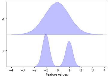
The plot_feature_histograms() function visualizes the distributions of all degrees of freedom assuming that the columns of data represent different features and the rows represent different time steps.

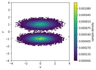
While plot_feature_histograms() can handle arbitrary numbers of features, we have additional plotting functions for 2D projections. First, we visualize the sample density in the \(x/y\)-plane…

fig, ax, misc = pyemma.plots.plot_density(*data.T)
ax.set_xlabel('$x$')
ax.set_ylabel('$y$')
ax.set_xlim(-4, 4)
ax.set_ylim(-4, 4)
ax.set_aspect('equal')
fig.tight_layout()

… then, we show the corresponding pseudo free energy surface:

fig, ax, misc = pyemma.plots.plot_free_energy(*data.T, legacy=False)
ax.set_xlabel('$x$')
ax.set_ylabel('$y$')
ax.set_xlim(-4, 4)
ax.set_ylim(-4, 4)
ax.set_aspect('equal')
fig.tight_layout()

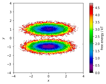
Both functions make a two-dimensional histogram for the given features; the free energy surface is defined by the negative logarithm of the probability computed from the histogram counts.

⚠️ Please note that these functions visualize the density and free energy of the sampled data, not the equilibrium distribution of the underlying system. To account for nonequiblibrium data, you can supply frame-wise weights using the weights parameter. This will be covered in the follow-up Notebook 04 ➜ 📓.

Case 2: loading *.xtc files (alanine dipeptide)

To load molecular dynamics data from one of the standard file formats ( *.xtc), we need not only the actual simulation data, but a topology file, too. This might differ for other formats though.

pdb = mdshare.fetch('alanine-dipeptide-nowater.pdb', working_directory='data')
files = mdshare.fetch('alanine-dipeptide-*-250ns-nowater.xtc', working_directory='data')
print(pdb)
print(files)

data/alanine-dipeptide-nowater.pdb
['data/alanine-dipeptide-0-250ns-nowater.xtc', 'data/alanine-dipeptide-1-250ns-nowater.xtc', 'data/alanine-dipeptide-2-250ns-nowater.xtc']

We can have a look at the structure with the aid of NGLView. We load the PDB file into memory with mdtraj and visualize it. The widget will auto-close after 30 second; if you want to watch it again, please execute the cell below again.

widget = nglview.show_mdtraj(mdtraj.load(pdb))
p = TrajectoryPlayer(widget)
widget.add_ball_and_stick()
p.spin = True
def stop_spin():
    p.spin = False
    widget.close()
Timer(30, stop_spin).start()
widget

In PyEMMA, the featurizer is a central object that incorporates the system’s topology. We start by creating it using the topology file. Features are now easily computed by adding the target feature. If no feature is added, the featurizer will extract Cartesian coordinates.

feat = pyemma.coordinates.featurizer(pdb)

Now we pass the featurizer to the load function to extract the Cartesian coordinates from the trajectory files into memory. For real world examples one would prefer the source() function, because usually one has more data available than main memory in the workstation.

The warning about plain coordinates is triggered, because these coordinates will include diffusion as a dynamical process, which might not be what one is interested in. If the molecule of interest has been aligned to a reference prior the analysis, it is fine to use these coordinates, but we will see that there are better choices.

data = pyemma.coordinates.load(files, features=feat)
print('type of data:', type(data))
print('lengths:', len(data))
print('shape of elements:', data[0].shape)
print('n_atoms:', feat.topology.n_atoms)

/storage/mi/marscher/software/miniconda3/conda-bld/pyemma-doc_1607519340854/_h_env_placehold_placehold_placehold_placehold_placehold_placehold_placehold_placehold_placehold_placehold_placehold_placehold_placehold_placehold_placehold_placehold_placehold_pl/lib/python3.9/site-packages/pyemma/coordinates/data/featurization/featurizer.py:881: UserWarning: You have not selected any features. Returning plain coordinates.
  warnings.warn("You have not selected any features. Returning plain coordinates.")

type of data: <class 'list'>
lengths: 3
shape of elements: (250000, 66)
n_atoms: 22

Next, we start adding features which we want to extract from the simulation data. Here, we want to load the backbone torsions, because these angles are known to describe all flexibility in the system. Since this feature is two dimensional, it is also easier to visualize. Please note that, in complex systems, it is not trivial to visualize plain input features.

feat = pyemma.coordinates.featurizer(pdb)
feat.add_backbone_torsions(periodic=False)

⚠️ Please note that the trajectories have been aligned to a reference structure before. Since in that case we loose track of the periodic box, we have to switch off the periodic flag for the torsion angle computations. By default PyEMMA assumes your simulation uses periodic boundary conditions.

We can always call the featurizer’s describe() method to show which features are requested. You might have noticed that you can combine arbitrary features by having multiple calls to add_ methods of the featurizer.

data = pyemma.coordinates.load(files, features=feat)

print('type of data:', type(data))
print('lengths:', len(data))
print('shape of elements:', data[0].shape)

type of data: <class 'list'>
lengths: 3
shape of elements: (250000, 2)

After we have selected all desired features, we can call the load() function to load all features into memory or, alternatively, the source() function to create a streamed feature reader. For now, we will use load():

print(feat.describe())

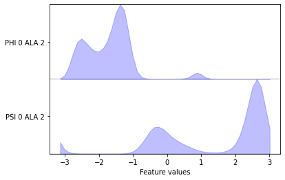
['PHI 0 ALA 2', 'PSI 0 ALA 2']

Apparently, we have loaded a list of three two-dimensional numpy.ndarray objects from our three trajectory files. We can visualize these features using the aforementioned plotting functions, but to do so we have to concatenate the three individual trajectories:

data_concatenated = np.concatenate(data)
pyemma.plots.plot_feature_histograms(data_concatenated, feature_labels=feat);

(<Figure size 432x288 with 1 Axes>, <AxesSubplot:xlabel='Feature values'>)

We can now measure the quantity of kinetic variance of the just selected feature by computing a VAMP-2 score wu-17. This enables us to distinguish features on how well they might be suited for MSM building. The minimum value of this score is \(1\), which corresponds to the invariant measure or the observed equilibrium.

With the dimension parameter we specify the amount of dynamic processes that we want to score. This is of importance later on, when we want to compare different input features (Notebook 02 ➜ 📓). If we did not fix this number, we would not have an upper bound for the score.

⚠️ Please also note that we split our available data into training and test sets, where we leave out the last file in training and then use it as test. This is an important aspect in practice to avoid over-fitting the score.

score_phi_psi = pyemma.coordinates.vamp(data[:-1], dim=2).score(
        test_data=data[-1],
        score_method='VAMP2')
print('VAMP2-score backbone torsions: {:.2f}'.format(score_phi_psi))

VAMP2-score backbone torsions: 1.50

The score of \(1.5\) means that we have the constant of \(1\) plus a total contribution of \(0.5\) from the other dynamic processes.

We now use PyEMMA’s plot_density() and plot_free_energy() functions to create Ramachandran plots of our system:

fig, axes = plt.subplots(1, 2, figsize=(10, 4), sharex=True, sharey=True)
# the * operator used in a function call is used to unpack
# the iterable variable into its single elements.
pyemma.plots.plot_density(*data_concatenated.T, ax=axes[0])
pyemma.plots.plot_free_energy(*data_concatenated.T, ax=axes[1], legacy=False)
for ax in axes.flat:
    ax.set_xlabel('$\Phi$')
    ax.set_aspect('equal')
axes[0].set_ylabel('$\Psi$')
fig.tight_layout()

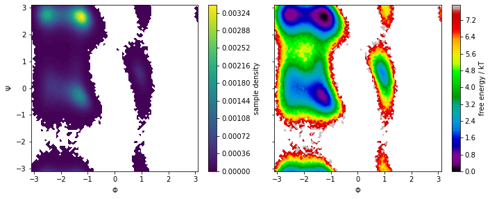
We note that the distribution in backbone torsion space contains several basins that will be assigned to metastable states in follow-up notebooks (Notebook 05 ➜ 📓, Notebook 07 ➜ 📓). Again, the free energy plot only depicts a pseudo free energy surface of the sampled data and was not re-weighted to equilibrium.

Let us look at a different featurization example and load the positions of all heavy atoms instead. We create a new featurizer object and use its add_selection() method to request the positions of a given selection of atoms. For this selection, we can use the select_Heavy() method which returns the indices of all heavy atoms.

Again, we load the data into memory and show what we loaded using the describe() method:

feat = pyemma.coordinates.featurizer(pdb)
feat.add_selection(feat.select_Heavy())

data = pyemma.coordinates.load(files, features=feat)

feat.describe()

['ATOM:ACE 1 CH3 1 x',
 'ATOM:ACE 1 CH3 1 y',
 'ATOM:ACE 1 CH3 1 z',
 'ATOM:ACE 1 C 4 x',
 'ATOM:ACE 1 C 4 y',
 'ATOM:ACE 1 C 4 z',
 'ATOM:ACE 1 O 5 x',
 'ATOM:ACE 1 O 5 y',
 'ATOM:ACE 1 O 5 z',
 'ATOM:ALA 2 N 6 x',
 'ATOM:ALA 2 N 6 y',
 'ATOM:ALA 2 N 6 z',
 'ATOM:ALA 2 CA 8 x',
 'ATOM:ALA 2 CA 8 y',
 'ATOM:ALA 2 CA 8 z',
 'ATOM:ALA 2 CB 10 x',
 'ATOM:ALA 2 CB 10 y',
 'ATOM:ALA 2 CB 10 z',
 'ATOM:ALA 2 C 14 x',
 'ATOM:ALA 2 C 14 y',
 'ATOM:ALA 2 C 14 z',
 'ATOM:ALA 2 O 15 x',
 'ATOM:ALA 2 O 15 y',
 'ATOM:ALA 2 O 15 z',
 'ATOM:NME 3 N 16 x',
 'ATOM:NME 3 N 16 y',
 'ATOM:NME 3 N 16 z',
 'ATOM:NME 3 C 18 x',
 'ATOM:NME 3 C 18 y',
 'ATOM:NME 3 C 18 z']

⚠️ Please note that PyEMMA has flattened the \(x, y\) and \(z\) coordinates into an array that will be used for further analysis.

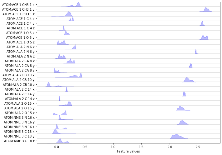
We visualize the distributions of all loaded features:

fig, ax = plt.subplots(figsize=(10, 7))
pyemma.plots.plot_feature_histograms(np.concatenate(data), feature_labels=feat, ax=ax)
fig.tight_layout()

Again we have a look at the VAMP-2 score of the heavy atom coordinates.

score_heavy_atoms = pyemma.coordinates.vamp(data[:-1], dim=2).score(
        test_data=data[:-1],
        score_method='VAMP2')
print('VAMP2-score backbone torsions: {:f}'.format(score_phi_psi))
print('VAMP2-score xyz: {:f}'.format(score_heavy_atoms))

VAMP2-score backbone torsions: 1.502240
VAMP2-score xyz: 2.471292

As we see, the score for the heavy atom positions is much higher as the one for the \(\phi/\psi\) torsion angles. The feature with a higher score should be favored for further analysis, because it means that this feature contains more information about slow processes. If you are already digging deeper into your system of interest, you can of course restrict the analysis to a set of features you already know describes your processes of interest, regardless of its VAMP score.

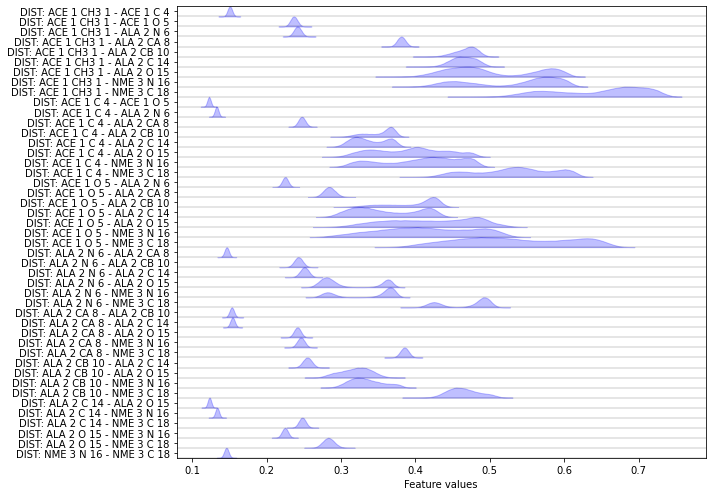
Another featurization that is interesting especially for proteins are pairwise heavy atom distances:

feat = pyemma.coordinates.featurizer(pdb)
heavy_atom_distance_pairs = feat.pairs(feat.select_Heavy())
feat.add_distances(heavy_atom_distance_pairs, periodic=False)
data = pyemma.coordinates.load(files, features=feat)

feat.describe()

['DIST: ACE 1 CH3 1 - ACE 1 C 4',
 'DIST: ACE 1 CH3 1 - ACE 1 O 5',
 'DIST: ACE 1 CH3 1 - ALA 2 N 6',
 'DIST: ACE 1 CH3 1 - ALA 2 CA 8',
 'DIST: ACE 1 CH3 1 - ALA 2 CB 10',
 'DIST: ACE 1 CH3 1 - ALA 2 C 14',
 'DIST: ACE 1 CH3 1 - ALA 2 O 15',
 'DIST: ACE 1 CH3 1 - NME 3 N 16',
 'DIST: ACE 1 CH3 1 - NME 3 C 18',
 'DIST: ACE 1 C 4 - ACE 1 O 5',
 'DIST: ACE 1 C 4 - ALA 2 N 6',
 'DIST: ACE 1 C 4 - ALA 2 CA 8',
 'DIST: ACE 1 C 4 - ALA 2 CB 10',
 'DIST: ACE 1 C 4 - ALA 2 C 14',
 'DIST: ACE 1 C 4 - ALA 2 O 15',
 'DIST: ACE 1 C 4 - NME 3 N 16',
 'DIST: ACE 1 C 4 - NME 3 C 18',
 'DIST: ACE 1 O 5 - ALA 2 N 6',
 'DIST: ACE 1 O 5 - ALA 2 CA 8',
 'DIST: ACE 1 O 5 - ALA 2 CB 10',
 'DIST: ACE 1 O 5 - ALA 2 C 14',
 'DIST: ACE 1 O 5 - ALA 2 O 15',
 'DIST: ACE 1 O 5 - NME 3 N 16',
 'DIST: ACE 1 O 5 - NME 3 C 18',
 'DIST: ALA 2 N 6 - ALA 2 CA 8',
 'DIST: ALA 2 N 6 - ALA 2 CB 10',
 'DIST: ALA 2 N 6 - ALA 2 C 14',
 'DIST: ALA 2 N 6 - ALA 2 O 15',
 'DIST: ALA 2 N 6 - NME 3 N 16',
 'DIST: ALA 2 N 6 - NME 3 C 18',
 'DIST: ALA 2 CA 8 - ALA 2 CB 10',
 'DIST: ALA 2 CA 8 - ALA 2 C 14',
 'DIST: ALA 2 CA 8 - ALA 2 O 15',
 'DIST: ALA 2 CA 8 - NME 3 N 16',
 'DIST: ALA 2 CA 8 - NME 3 C 18',
 'DIST: ALA 2 CB 10 - ALA 2 C 14',
 'DIST: ALA 2 CB 10 - ALA 2 O 15',
 'DIST: ALA 2 CB 10 - NME 3 N 16',
 'DIST: ALA 2 CB 10 - NME 3 C 18',
 'DIST: ALA 2 C 14 - ALA 2 O 15',
 'DIST: ALA 2 C 14 - NME 3 N 16',
 'DIST: ALA 2 C 14 - NME 3 C 18',
 'DIST: ALA 2 O 15 - NME 3 N 16',
 'DIST: ALA 2 O 15 - NME 3 C 18',
 'DIST: NME 3 N 16 - NME 3 C 18']

Now let us compare the score of heavy atom distance pairs to the other scores.

score_pair_heavy_atom_dists = pyemma.coordinates.vamp(data[:-1], dim=2).score(
    test_data=data[-1],
    score_method='VAMP2')
print('VAMP2-score: {:.2f}'.format(score_pair_heavy_atom_dists))

VAMP2-score: 2.40

Apparently, the heavy atom distance pairs cover an amount of kinetic variance which is comparable to the coordinates themselves. However we probably would not use much information by using this internal degree of freedom, while avoiding the need to align our trajectories first.

load() versus source()

Using load(), we put the full data into memory. This is possible for all examples in this tutorial.

Many real world applications, though, require more memory than your workstation might provide. For these cases, you should use the source() function:

reader = pyemma.coordinates.source(files, features=feat)
print(reader)

<pyemma.coordinates.data.feature_reader.FeatureReader object at 0x7fadaa705d60>

This function creates a reader, wich allows to stream the underlying data in chunks instead of the full set. Most of the functions in the coordinates sub-package accept data in memory as well as readers. However, some plotting functions require the data to be in memory. To load a (sub-sampled) subset into memory, we can use the get_output() method with a stride parameter:

data_output = reader.get_output(stride=5)
len(data_output)
print('number of frames in first file: {}'.format(reader.trajectory_length(0)))
print('number of frames after striding: {}'.format(len(data_output[0])))

number of frames in first file: 250000
number of frames after striding: 50000

We now have loaded every fifth frame into memory. Again, we can visualize the (concatenated) features with a feature histogram:

fig, ax = plt.subplots(figsize=(10, 7))
pyemma.plots.plot_feature_histograms(
    np.concatenate(data_output), feature_labels=feat, ax=ax)
fig.tight_layout()

Testing your progress

In the remainder of this notebook, you will find short exercises to test your newly learned skills. The exercises are announced by the keyword Exercise and followed by an incomplete cell. Missing parts are indicated by

#FIXME

Exercise cells come with a button (Show Solution) to reveal the solution.

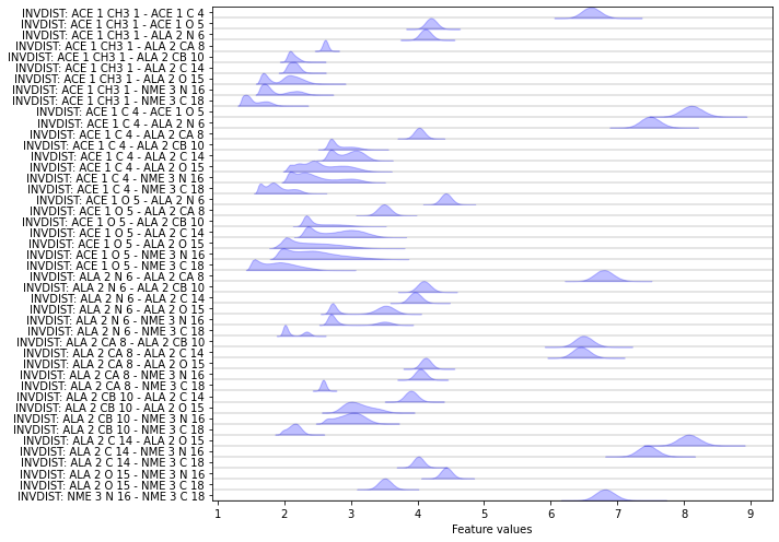
Exercise 1: inverse heavy atom distances

Please fix the following code block such that the inverse distances between all heavy atoms are loaded and visualized.

Hint: try to use the auto-complete feature on the feat object to gain some insight. Also take a look at the previous demonstrations.

Solution

feat = pyemma.coordinates.featurizer(pdb)
pairs = feat.pairs(feat.select_Heavy())
feat.add_inverse_distances(pairs)

data = pyemma.coordinates.load(files, features=feat)

fig, ax = plt.subplots(figsize=(10, 7))
pyemma.plots.plot_feature_histograms(
    np.concatenate(data), feature_labels=feat, ax=ax)

fig.tight_layout()

Excercise 2: compare the inverse distances feature to the previously computed ones

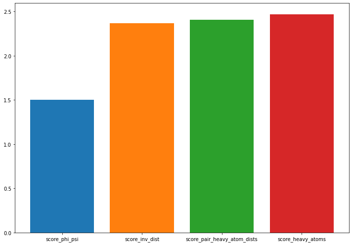
Compute and discuss a cross-validated VAMP score for the inverse pairwise heavy atom distances and plot the result. What do you observe and which feature would you choose for further processing?

Solution

score_inv_dist = pyemma.coordinates.vamp(
    data[:-1], dim=2).score(test_data=data[-1])

fig, ax = plt.subplots(figsize=(10, 7))
score_mapping = dict(score_heavy_atoms=score_heavy_atoms,
                     score_phi_psi=score_phi_psi,
                     score_pair_heavy_atom_dists=score_pair_heavy_atom_dists,
                     score_inv_dist=score_inv_dist)
lbl = []
for i, (key, value) in enumerate(sorted(score_mapping.items(), key=lambda x: x[1])):
    ax.bar(i, height=value)
    lbl.append(key)
ax.set_xticks(np.arange(0, len(score_mapping), 1))
ax.set_xticklabels(lbl)
fig.tight_layout()

Case 3: loading *.xtc files (pentapeptide)

Once we have obtained the raw data files…

pdb = mdshare.fetch('pentapeptide-impl-solv.pdb', working_directory='data')
files = mdshare.fetch('pentapeptide-*-500ns-impl-solv.xtc', working_directory='data')

… and had a quick look at the structure again…

widget = nglview.show_mdtraj(mdtraj.load(pdb))
p = TrajectoryPlayer(widget)
widget.add_ball_and_stick()
p.spin = True
def stop_spin():
    p.spin = False
    widget.close()
Timer(30, stop_spin).start()
widget

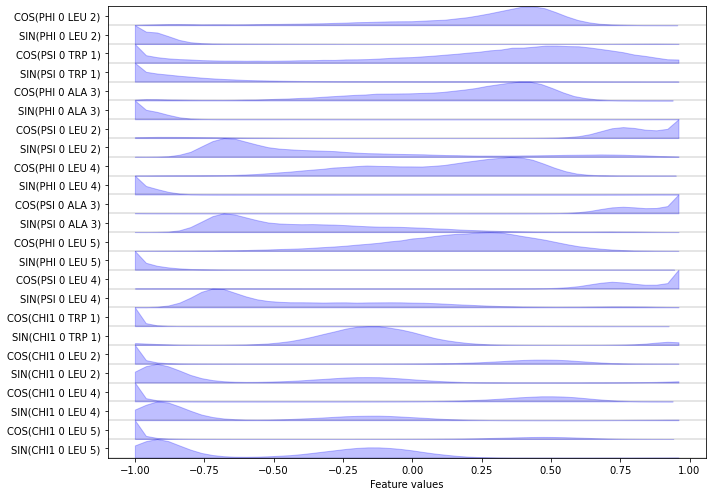
… we can load a selection of features into memory. Here, we want the \(\cos/\sin\) transformations of the backbone and \(\chi_1\) sidechain torsions.

feat = pyemma.coordinates.featurizer(pdb)
feat.add_backbone_torsions(cossin=True, periodic=False)
feat.add_sidechain_torsions(which='chi1', cossin=True, periodic=False)

data = pyemma.coordinates.load(files, features=feat)
data_concatenated = np.concatenate(data)

print(feat.describe())

/storage/mi/marscher/software/miniconda3/conda-bld/pyemma-doc_1607519340854/_h_env_placehold_placehold_placehold_placehold_placehold_placehold_placehold_placehold_placehold_placehold_placehold_placehold_placehold_placehold_placehold_placehold_placehold_pl/lib/python3.9/site-packages/mdtraj/geometry/dihedral.py:374: FutureWarning: arrays to stack must be passed as a "sequence" type such as list or tuple. Support for non-sequence iterables such as generators is deprecated as of NumPy 1.16 and will raise an error in the future.
  indices = np.vstack(x for x in indices if x.size)[id_sort]
/storage/mi/marscher/software/miniconda3/conda-bld/pyemma-doc_1607519340854/_h_env_placehold_placehold_placehold_placehold_placehold_placehold_placehold_placehold_placehold_placehold_placehold_placehold_placehold_placehold_placehold_placehold_placehold_pl/lib/python3.9/site-packages/pyemma/coordinates/data/featurization/angles.py:211: FutureWarning: arrays to stack must be passed as a "sequence" type such as list or tuple. Support for non-sequence iterables such as generators is deprecated as of NumPy 1.16 and will raise an error in the future.
  indices = np.vstack(valid.values())

['COS(PHI 0 LEU 2)', 'SIN(PHI 0 LEU 2)', 'COS(PSI 0 TRP 1)', 'SIN(PSI 0 TRP 1)', 'COS(PHI 0 ALA 3)', 'SIN(PHI 0 ALA 3)', 'COS(PSI 0 LEU 2)', 'SIN(PSI 0 LEU 2)', 'COS(PHI 0 LEU 4)', 'SIN(PHI 0 LEU 4)', 'COS(PSI 0 ALA 3)', 'SIN(PSI 0 ALA 3)', 'COS(PHI 0 LEU 5)', 'SIN(PHI 0 LEU 5)', 'COS(PSI 0 LEU 4)', 'SIN(PSI 0 LEU 4)', 'COS(CHI1 0 TRP 1)', 'SIN(CHI1 0 TRP 1)', 'COS(CHI1 0 LEU 2)', 'SIN(CHI1 0 LEU 2)', 'COS(CHI1 0 LEU 4)', 'SIN(CHI1 0 LEU 4)', 'COS(CHI1 0 LEU 5)', 'SIN(CHI1 0 LEU 5)']

Finally, we visualize the (concatenated) features:

fig, ax = plt.subplots(figsize=(10, 7))
pyemma.plots.plot_feature_histograms(data_concatenated, feature_labels=feat, ax=ax)
fig.tight_layout()

Exercises: feature selection and visualization

Exercise 3

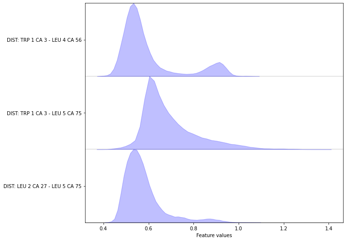
Complete the following code block to load/visualize the distances between all \(\text{C}_\alpha\) carbon atoms.

Hint: You might find the add_distances_ca() method of the featurizer object helpful.

Solution

feat = pyemma.coordinates.featurizer(pdb)
feat.add_distances_ca(periodic=False)

data = pyemma.coordinates.load(files, features=feat)
data_concatenated = np.concatenate(data)

fig, ax = plt.subplots(figsize=(10, 7))
pyemma.plots.plot_feature_histograms(data_concatenated, feature_labels=feat, ax=ax)
fig.tight_layout()

Exercise 4

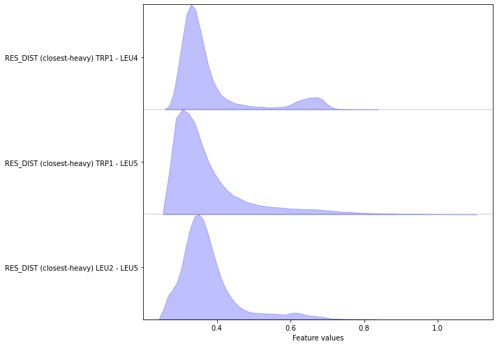
Complete the following code block to load/visualize the minimal distances between all residues (excluding first and second neighbors).

Hint: You might find the add_residue_mindist() method of the featurizer object helpful.

Solution

feat = pyemma.coordinates.featurizer(pdb)
feat.add_residue_mindist(periodic=False)

data = pyemma.coordinates.load(files, features=feat)
data_concatenated = np.concatenate(data)

fig, ax = plt.subplots(figsize=(10, 7))
pyemma.plots.plot_feature_histograms(data_concatenated, feature_labels=feat, ax=ax)
fig.tight_layout()

09-12-20 14:22:09 pyemma.coordinates.data.featurization.featurizer.MDFeaturizer[35] WARNING  Using all residue pairs with schemes like closest or closest-heavy is very time consuming. Consider reducing the residue pairs

WARNING:pyemma.coordinates.data.featurization.featurizer.MDFeaturizer[35]:Using all residue pairs with schemes like closest or closest-heavy is very time consuming. Consider reducing the residue pairs

Exercise 5

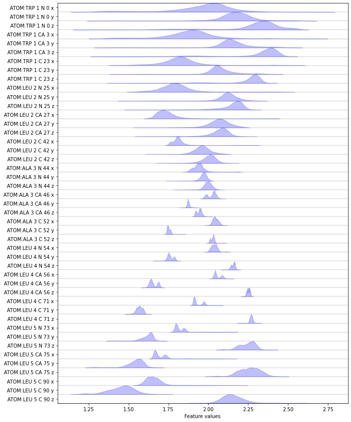
Complete the following code block to load/visualize the position of all backbone atoms.

Hint: You might find the select_Backbone() method of the featurizer object helpful.

Solution

feat = pyemma.coordinates.featurizer(pdb)
feat.add_selection(feat.select_Backbone())

data = pyemma.coordinates.load(files, features=feat)
data_concatenated = np.concatenate(data)

fig, ax = plt.subplots(figsize=(10, 12))
pyemma.plots.plot_feature_histograms(data_concatenated, feature_labels=feat, ax=ax)
fig.tight_layout()

Exercise 6

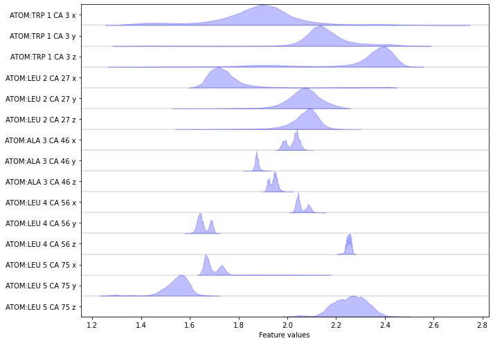
Complete the following code block to load/visualize the position of all \(\text{C}_\alpha\) atoms.

Hint: You might find the select_Ca() method of the featurizer object helpful.

Solution

feat = pyemma.coordinates.featurizer(pdb)
feat.add_selection(feat.select_Ca())

data = pyemma.coordinates.load(files, features=feat)
data_concatenated = np.concatenate(data)

fig, ax = plt.subplots(figsize=(10, 7))
pyemma.plots.plot_feature_histograms(data_concatenated, feature_labels=feat, ax=ax)
fig.tight_layout()

Wrapping up

In this notebook, we have learned how to load and visualize molecular simulation data with PyEMMA. In detail, we have used - pyemma.coordinates.featurizer() to define a selection of features we want to extract, - pyemma.coordinates.load() to load data into memory, and - pyemma.coordinates.source() to create a streamed feature reader in case the data does not fit into memory.

After loading the data into memory, we have used - pyemma.coordinates.vamp().score() to score the quality of the features, - pyemma.plots.plot_feature_histograms() to show the distributions of all loaded features, - pyemma.plots.plot_density() to visualize the sample density, and - pyemma.plots.plot_free_energy() to visualize the free energy surface of two selected features.

References

[^]Wu, H. and Noé, F.. 2017. Variational approach for learning Markov processes from time series data. URL