Augmented Markov models, a walk-through tutorial

Author: Simon Olsson (simon.olsson@fu-berlin.de) [@smnlssn](http://twitter.com/smnlssn)

Dec 2017-Jan 2018

Augmented Markov models (AMM) are a flavor of Markov state models (MSM) which take into account experimental data during model estimation. Using AMMs we can partially compensate for systematic errors in empirical MD forcefields or equivalently in coarse-grained models, and thereby hopefully get more accurate physical descriptions of thermodynamics and molecular kinetics of molecular systems.

In our recent paper we present the first statistical estimator of its kind, which allows for the integration of stationary expectation values as restraints. By stationary expectation value we mean

\[\mathbf{o} = \int \mathrm{d}x\; o(x)p(x)\, , \; \, \, \, \, \,p(x)=\mathcal{Z}^{-1}\exp(-\beta E(x))\]

where \(\mathbf{o}\) is an experimentally measured value, \(o(x)\) is a ‘forward model’ which back-computes a micro-scopic, instantaneous value of the experimental observable. Below we will given an example of such a forward model, the Karplus equation. \(p(x)\) is the Boltzmann distribution corresponding to the potential energy function \(E(x)\) and \(x\) is a molecular configuration. Consequently, these observables are time and ensemble averages over a large number of molecules, such as those obtained in bulk experiments including NMR spectroscopy.

Although we currently only allow for integration of stationary observables, we anticipate to extend support to dynamic observables in the near future. In the mean-time dynamic observables from experiments such as FRET and NMR Relaxation dispersion may be used for validation. We show an example of this in the end of this notebook

Special thanks to Tim Hempel, Andreas Mardt and Fabian Paul for comments on early versions of this notebook.

Prerequisites

In this tutorial I assume some familiarity with MSM theory and possibly also some practical experience, such as going through this PyEMMA tutorial. I recommend working your way through this tutorial if you are not already familiar with MSMs or if you are not familiar with PyEMMA.

Technical requirements

• Python 3

• PyEMMA 2.5

• Numpy

• matplotlib

Content of this notebook

• A quick primer to AMMs using a simple 1D double-well potential

• Using experimental J-couplings and MD simulations to build an AMM of the protein GB3

• Sanity checks and hyper-parameter optimization

%matplotlib inline
import pyemma as pe
from pyemma.datasets import double_well_discrete
import numpy as np
from matplotlib import pyplot as plt
import matplotlib as mpl

print("PyEMMA version", pe.version)
print("numpy version", np.version.full_version)
print("matplotlib version", mpl.__version__)

PyEMMA version 2.4+529.g43a3c781.dirty
numpy version 1.13.1
matplotlib version 2.0.2

Preparation of double-well data

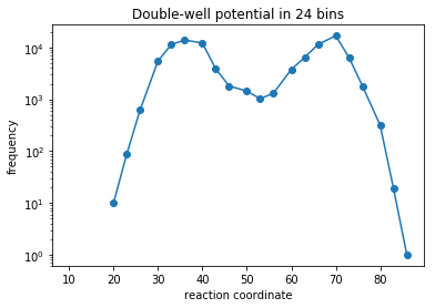
We extract pre-generated data from a double-well potential and discretize it into 20 evenly sized bins. In a practical setting of a molecular system one would perform dimensionalty reduction of some molecular features, cluster the simulation data in this space, and then use use the discretized trajectories down-stream.

double_well_data = double_well_discrete.DoubleWell_Discrete_Data()
reaction_coordinate = np.linspace(10,90,25, dtype='int')[:-1]
discrete_trajectory_20bins = double_well_data.dtraj_T100K_dt10_n(np.linspace(10,90,25, dtype='int').tolist())

plt.semilogy(reaction_coordinate, np.bincount(discrete_trajectory_20bins),'o-')
plt.xlabel('reaction coordinate')
plt.ylabel('frequency')
plt.title('Double-well potential in %i bins'%(len(np.bincount(discrete_trajectory_20bins))))

<matplotlib.text.Text at 0x11a339550>

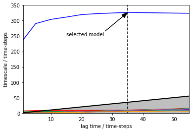
Selecting a suitable Markov state model

Plotting implied time-scales and selecting the model with lag-time of 35 time-steps

lags = [1,5,10,15,20,25,35,50,55]
implied_ts = pe.msm.its(dtrajs=discrete_trajectory_20bins,lags=lags)
pe.plots.plot_implied_timescales(implied_ts,units='time-steps', ylog=False)
plt.vlines(35,ymin=0,ymax=350,linestyles='dashed')
plt.annotate("selected model", xy=(lags[-3], implied_ts.timescales[-3][0]), xytext=(15,250),
                 arrowprops=dict(facecolor='black', shrink=0.001, width=0.1,headwidth=8))
plt.ylim([0,350])

100%|██████████| 9/9 [00:01<00:00,  5.27it/s]

(0, 350)

M = pe.msm.estimate_markov_model(dtrajs=discrete_trajectory_20bins, lag = lags[-3])

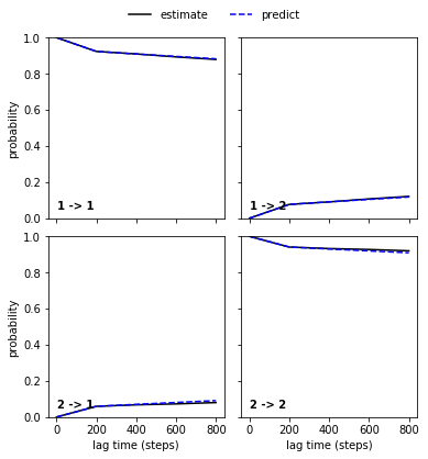
Performing a Chapman-Kolmogorov test

The Chapman-Kolmogorov test checks whether the MSM we have build makes predictions which are consisent with direct estimates from our simulation data. The test is based upon the Chapman-Kolmogorov equation which in the context of Markov models can be written as

\[\underbrace{T(K\tau)}_{\text{black line}} = \underbrace{T(\tau)^K}_{\text{blue dashed line}}\]

which states that transition matrix estimated at lag-time \(\tau\) to the \(K\)’th power should be equal to a transition matrix estimated at lag-time \(K\tau\). Therefore, if we have built a good MSM the two lines will be close in the plot below:

cktest = M.cktest(nsets=2)

100%|██████████| 9/9 [00:01<00:00,  5.12it/s]

cktplt = pe.plots.plot_cktest(cktest)

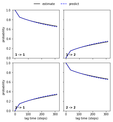
Looks good!

Experimental observables

Now, let’s check agreement with some synthetic experimental value which depends on our reaction coordinate from above.

First we compute the observable for each discrete states in our simulation data. Here, we map each bin on our axis to a point in the range \(\theta \in [0,\pi]\) and compute a faux experimental J-coupling observable using the Karplus equation,

\[^3J(\theta) = 3.2\cos^2(\theta) - 1.3\cos(\theta) + 4.2.\]

The Karplus equation is an example of a forward model, which maps a molecular feature – in this case a dihedral angle – to an experimental observable, here the \(^3\)J-coupling or scalar coupling.

_theta = np.linspace(0, np.pi, len(reaction_coordinate))
f_obs = 3.2*np.cos(_theta)**2 - 1.3*np.cos(_theta) + 4.2

In the case of a molecular system, one would compute some observable of interest for all the frames in our molecular simulation, and then average the predicted observable in each cluster/Markov state. But more about that below …

We can use the expectation method of our PyEMMA MSM instance to compute weighted ensemble averages:

print("Our simulated J-coupling is: %1.1fHz"%M.expectation(f_obs[M.active_set]).round(2))

Our simulated J-coupling is: 5.5Hz

Note how we have selected a subset (M.active_set) of the original clusters/discrete states. We do this, as there is no gaurantee that the MSM describes all of the states well. In general, PyEMMA finds the ‘largest connected set’, which is the larget set of clusters which we have both entered and exited.

Say we have measured an experimental value, which is 4.1Hz with an uncertainty of 0.8Hz. In such a case, we have a clear discrepancy between the predicted and experimental values. In these cases we can use AMMs to hopefully improve the model. With PyEMMA it is easy to try this out once you have established a regular Markov state model.

First we compute the experimental observable for all our simulation frames and store them in ftrajs

ftrajs = f_obs[discrete_trajectory_20bins].reshape(-1,1)

Then we have a convienence function estimate_augmented_markov_model to estimate AMMs by simply providing the ftraj, experimental averages and uncertainties:

AMM = pe.msm.estimate_augmented_markov_model(
    dtrajs = [discrete_trajectory_20bins], #Discrete trajectories as for the MSM
    ftrajs = [ftrajs], #Trajectories projected onto experimental observable
    lag = lags[-3],  # same lag-time as the one validated for the MSM
    m = np.array([4.1]),  # experimental average
    sigmas = np.array([0.8]), # experimental uncertainty
    maxiter=50000) # Maximum number of iterations

04-01-18 00:33:43 pyemma.msm.estimators.maximum_likelihood_msm.AugmentedMarkovModel[2] INFO     Total experimental constraints outside support 0 of 1
04-01-18 00:33:43 pyemma.msm.estimators.maximum_likelihood_msm.AugmentedMarkovModel[2] INFO     Converged Lagrange multipliers after 234 steps...
04-01-18 00:33:43 pyemma.msm.estimators.maximum_likelihood_msm.AugmentedMarkovModel[2] INFO     Converged pihat after 234 steps...

That is it!

We get some useful information as output here: All our experimental data are within the support, ie. the range of our observable sampled during the MD simulations. Lagrange multipliers and biased ensemble estimate both converged after 2 iterations.

Let’s compare the stationary properties of our AMM with the corresponding MSM.

bias_potential=np.exp(AMM.lagrange[0]*f_obs[M.active_set])
bias_potential=bias_potential/bias_potential.sum()

fig,ax=plt.subplots(ncols=2,figsize=(8,3))
ax[0].semilogy(_theta[AMM.active_set], AMM.stationary_distribution,'-o',label='AMM')
ax[0].semilogy(_theta[M.active_set], M.stationary_distribution, label='MSM')
ax[0].set_xlabel(r'$\theta\, /\, \mathrm{rad}$')
ax[0].set_ylabel(r'$p(\theta)$')
ax[1].semilogy(f_obs[AMM.active_set], AMM.stationary_distribution,'-o',label='AMM')
ax[1].semilogy(f_obs[M.active_set], M.stationary_distribution, label='MSM')
ax[1].semilogy(f_obs[M.active_set], bias_potential,'--', label='Experimental bias')
ax[1].set_xlabel(r'$^3J\, /\, \mathrm{Hz}$')
ax[1].set_ylabel(r'$p(^3J)$')
ax[1].legend()
plt.tight_layout()

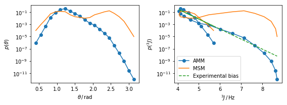
The plots above show the AMM stationary distribution versus the \(\theta\) and \(^3J\) variables defined above. The dashed green line in the plot on the right shows the bias introduced by the experimental data. The slope of this curve is given by the Lagrange multiplier estimated. Note how the distribution in our observable space \(p(^3J)\) maps different \(\theta\)-values to similar values, this causes of the knotted appearence of the curve.

We can also check whether we are closer to the experimental - drumroll …

print("Our AMM J-coupling is: %1.1fHz"%AMM.expectation(f_obs[AMM.active_set]).round(2))

Our AMM J-coupling is: 4.2Hz

Which closer to our ‘experimental’ average of 4.1Hz.

Try to play around with the experimental average and uncertainty to get some intuition how the AMM estimator changes the stationary properties as a function these parameters.

Bonus information for advanced users

Instead of using the convienence function above we can also build AMM instances directly. In this manner we have more flexibility in terms of input and manipulation of the object before actually estimating the AMM. We may for instance use an E-matrix as a way to input our predicted observables for each Markov state. This matrix must have the dimensions number_of_discrete_states times number_of_experimental_observables. An example of how to compute such a matrix can be found below. Note how we here specify a weight \(w\) instead of the uncertainties \(\sigma\) – they are related as \(\sigma = \sqrt{\frac{1}{2w}}\).

AMM_Advanced_inst = pe.msm.AugmentedMarkovModel(lag=lags[-3],
                                           E = AMM.E, #Average experimental observable in each discrete state
                                           m = np.array([4.1]),
                                           w = np.array([1./2./0.8**2]),
                                           maxiter = 50000
                                          )
AMM_Advanced_est = AMM_Advanced_inst.estimate(discrete_trajectory_20bins)

04-01-18 00:33:44 pyemma.msm.estimators.maximum_likelihood_msm.AugmentedMarkovModel[3] INFO     Total experimental constraints outside support 0 of 1
04-01-18 00:33:44 pyemma.msm.estimators.maximum_likelihood_msm.AugmentedMarkovModel[3] INFO     Converged Lagrange multipliers after 234 steps...
04-01-18 00:33:44 pyemma.msm.estimators.maximum_likelihood_msm.AugmentedMarkovModel[3] INFO     Converged pihat after 234 steps...

print("We check whether the results are consistent:",np.allclose(AMM_Advanced_est.stationary_distribution, AMM.stationary_distribution))

We check whether the results are consistent: True

AMM of GB3

To illustrate the use of AMMs for a small molecular system, we turn to GB3. We use back-bone torsions from a number of residues previously shown to be flexible. Below we execute the following protocol:

• We featurize 35 short MD trajectories,

• Perform TICA dimensionality reduction to 2 dimensions

• Cluster to 112 cluster centers

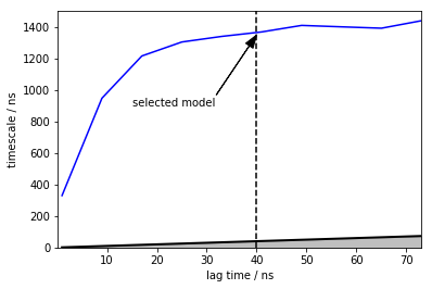
• Select a MSM with lag-time 40 nanoseconds (based upon an implied time-scale plot and a CK test above.)

Please note that this data-set is relatively small (~14 microseconds) and uncertainties of the quantities therefore will be large. For illustrative purposes we will not dwell on this point further in this tutorial.

feat = pe.coordinates.featurizer("gb3_data/gb3_backbone_top.pdb")

for ri in [8,9,10,11,12,13,14,36,37,38,39,40,41]:
    feat.add_backbone_torsions(selstr='residue %i'%ri, cossin=True)

source = pe.coordinates.source(['gb3_data/gb3_backbone_{:03d}.xtc'.format(i) for i in range(35)], features=feat)

100%|██████████| 35/35 [00:00<00:00, 315.85it/s]

lag=55
tica_obj = pe.coordinates.tica(source, lag=lag, dim=2)

Y = tica_obj.get_output() # get tica coordinates

100%|██████████| 35/35 [00:02<00:00, 19.09it/s]
100%|██████████| 35/35 [00:01<00:00, 22.83it/s]

pe.config.show_progress_bars = False
Y_all = np.vstack(Y)
n_clusters = 112 # number of k-means clusters

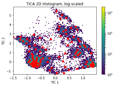
clustering = pe.coordinates.cluster_kmeans(Y, k = n_clusters, max_iter = 100, stride = 10)

dtrajs = clustering.assign(Y)

cx = clustering.clustercenters[:,0]
cy = clustering.clustercenters[:,1]

plt.hist2d(Y_all[:, 0], Y_all[:, 1], bins=100, norm = mpl.colors.LogNorm())
plt.colorbar()
plt.scatter(cx, cy,  marker='o',  color='red')
plt.xlabel('TIC 1')
plt.ylabel('TIC 2')
plt.title('TICA 2D Histogram, log-scaled')

04-01-18 00:34:11 pyemma.coordinates.clustering.kmeans.KmeansClustering[6] INFO     Cluster centers converged after 11 steps.

<matplotlib.text.Text at 0x11ec03e10>

Model selection and self-consitency checks

time_step_ps = 200
lags = range(5,400,40)
its = pe.msm.its(dtrajs, lags=lags, nits=1, reversible=True)

pe.plots.plot_implied_timescales(its, ylog = False, dt=time_step_ps*1e-3, units='ns')
plt.vlines(40,ymin=0,ymax=1500,linestyles='dashed')
plt.annotate("selected model", xy=(40, 1350), xytext=(15,900),
                 arrowprops=dict(facecolor='black', shrink=0.001, width=0.1,headwidth=8))
plt.ylim([0,1500])

(0, 1500)

M_gb3 = pe.msm.estimate_markov_model(dtrajs, lag=200)

ckt_gb3 = M_gb3.cktest(2, mlags=5)

pe.plots.plot_cktest(ckt_gb3)

(<matplotlib.figure.Figure at 0x124611b38>,
 array([[<matplotlib.axes._subplots.AxesSubplot object at 0x12481e358>,
         <matplotlib.axes._subplots.AxesSubplot object at 0x11f29b0f0>],
        [<matplotlib.axes._subplots.AxesSubplot object at 0x11f242ac8>,
         <matplotlib.axes._subplots.AxesSubplot object at 0x11f287f60>]], dtype=object))

Computation of scalar couplings from simulation data

We use a dataset of HN-HA scalar couplings and Karplus parameters from this paper to test the quality of our MSM. This observable is sensitive to the ensemble of sampled \(\phi\) angles.

#Karplus parameters
A_ = 8.754
B_ = -1.222
C_ = 0.111

# Load data
expljc = np.loadtxt('gb3_data/HN_HA_JC.dat')

# Get all phi-angles
feat_jcoupl = pe.coordinates.featurizer(topfile='gb3_data/gb3_backbone_top.pdb')
feat_jcoupl.add_backbone_torsions()
phi_indices = [i for i,st in enumerate(feat_jcoupl.describe()) if "PHI" in st]
md_phi_rindex=[int(a.split(" ")[-1]) for a in np.array(feat_jcoupl.describe())[phi_indices].tolist()]
sourcejc = pe.coordinates.source(['gb3_data/gb3_backbone_{:03d}.xtc'.format(i) for i in range(35)], features=feat_jcoupl)
phis_ = [dih[:, phi_indices] for dih in sourcejc.get_output() ]

#Compute scalar-couplings
Phi_all = np.vstack(phis_)-np.pi/3 # correct the phase
cosPhi_all = np.cos(Phi_all)
cossqPhi_all = cosPhi_all*cosPhi_all
JC_all = A_*cossqPhi_all+B_*cosPhi_all+C_

Compute E-matrix

# Compute E-matrix
dta = np.concatenate(dtrajs) # concatenate our discretized trajectories
all_markov_states = set(dta) # get set set of all possible states
_E = np.zeros((len(all_markov_states), JC_all.shape[1])) # initialize E-matrix
for i, s in enumerate(all_markov_states): # loop over all Markov states
    _E[i, :] = JC_all[np.where(dta == s)].mean(axis = 0) # compute average observable over Markov state i

#Find intersection in set of computable and measured scalar couplings.
a=[int(i) for i in set(md_phi_rindex).intersection(expljc[:,0])]
idx_expl = [np.where(expljc[:,0]==i)[0][0] for i in a]
idx_md = [np.where(np.array(md_phi_rindex)==i)[0][0] for i in a]

plt.plot(np.array(md_phi_rindex)[idx_md], M_gb3.stationary_distribution.dot(_E[:, idx_md]),'o',label='MSM')
plt.plot(expljc[idx_expl,0], expljc[idx_expl,1],'x', label='Experiment')
plt.xlabel('residue index')
plt.ylabel(r'$^3J_{\mathrm{H}^{\mathrm{N}}-\mathrm{H}^{\alpha}}\, / \, \mathrm{Hz}$')
plt.title(r'Comparison of MSM predictions with $^3J_{\mathrm{H}^{\mathrm{N}}-\mathrm{H}^{\alpha}}$ data')
plt.legend()

<matplotlib.legend.Legend at 0x124334be0>

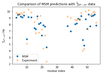
In general, we observe a fair qualitative agreement with the data. However, considering the upper error of 0.3Hz has been reported for these data a quantitative agreement is clearly missing.

#Setup input for AMM estimation
ftrajs = np.split(JC_all[:, idx_md], np.cumsum([len(p) for p in phis_])[:-1], axis=0)
expl_data = expljc[idx_expl, 1].reshape(-1)
expl_sigmas = 0.3*np.ones(expl_data.shape)

# We increase the uncertainty for a subset of the data to illustrate non-uniform errors
expl_sigmas[18:21] = expl_sigmas[18:21] + 0.5

amm_gb3 = pe.msm.estimate_augmented_markov_model(dtrajs = dtrajs,
                                                 ftrajs = ftrajs,
                                                 lag = 200,
                                                 m = expl_data,
                                                 sigmas = expl_sigmas
                                                )

04-01-18 00:34:27 pyemma.msm.estimators.maximum_likelihood_msm.AugmentedMarkovModel[10] INFO     Experimental value 9.773668 is outside the support (8.864312,9.617295)
04-01-18 00:34:27 pyemma.msm.estimators.maximum_likelihood_msm.AugmentedMarkovModel[10] INFO     Experimental value 9.678525 is outside the support (8.688147,9.656137)
04-01-18 00:34:27 pyemma.msm.estimators.maximum_likelihood_msm.AugmentedMarkovModel[10] INFO     Experimental value 9.735873 is outside the support (7.894706,9.565636)
04-01-18 00:34:27 pyemma.msm.estimators.maximum_likelihood_msm.AugmentedMarkovModel[10] INFO     Experimental value 9.571859 is outside the support (8.513741,9.428110)
04-01-18 00:34:27 pyemma.msm.estimators.maximum_likelihood_msm.AugmentedMarkovModel[10] INFO     Experimental value 9.898549 is outside the support (8.409517,9.767085)
04-01-18 00:34:27 pyemma.msm.estimators.maximum_likelihood_msm.AugmentedMarkovModel[10] INFO     Experimental value 5.083449 is outside the support (5.162310,6.510399)
04-01-18 00:34:27 pyemma.msm.estimators.maximum_likelihood_msm.AugmentedMarkovModel[10] INFO     Experimental value 10.289247 is outside the support (8.668080,9.411788)
04-01-18 00:34:27 pyemma.msm.estimators.maximum_likelihood_msm.AugmentedMarkovModel[10] INFO     Experimental value 9.841005 is outside the support (8.114074,9.749027)
04-01-18 00:34:27 pyemma.msm.estimators.maximum_likelihood_msm.AugmentedMarkovModel[10] INFO     Experimental value 8.359442 is outside the support (6.155785,8.071151)
04-01-18 00:34:27 pyemma.msm.estimators.maximum_likelihood_msm.AugmentedMarkovModel[10] INFO     Experimental value 6.783495 is outside the support (7.617393,8.474687)
04-01-18 00:34:27 pyemma.msm.estimators.maximum_likelihood_msm.AugmentedMarkovModel[10] INFO     Experimental value 9.351349 is outside the support (7.728871,8.916314)
04-01-18 00:34:27 pyemma.msm.estimators.maximum_likelihood_msm.AugmentedMarkovModel[10] INFO     Experimental value 7.265520 is outside the support (5.625987,6.574851)
04-01-18 00:34:27 pyemma.msm.estimators.maximum_likelihood_msm.AugmentedMarkovModel[10] INFO     Experimental value 4.320463 is outside the support (7.365972,8.813777)
04-01-18 00:34:27 pyemma.msm.estimators.maximum_likelihood_msm.AugmentedMarkovModel[10] INFO     Experimental value 6.322209 is outside the support (6.639600,8.443197)
04-01-18 00:34:27 pyemma.msm.estimators.maximum_likelihood_msm.AugmentedMarkovModel[10] INFO     Experimental value 2.378610 is outside the support (4.092054,5.080344)
04-01-18 00:34:27 pyemma.msm.estimators.maximum_likelihood_msm.AugmentedMarkovModel[10] INFO     Experimental value 9.206853 is outside the support (4.378050,9.200555)
04-01-18 00:34:27 pyemma.msm.estimators.maximum_likelihood_msm.AugmentedMarkovModel[10] INFO     Experimental value 8.725843 is outside the support (6.703235,8.699459)
04-01-18 00:34:27 pyemma.msm.estimators.maximum_likelihood_msm.AugmentedMarkovModel[10] INFO     Experimental value 9.778475 is outside the support (8.256344,9.650097)
04-01-18 00:34:27 pyemma.msm.estimators.maximum_likelihood_msm.AugmentedMarkovModel[10] INFO     Experimental value 4.034841 is outside the support (5.142444,6.329253)
04-01-18 00:34:27 pyemma.msm.estimators.maximum_likelihood_msm.AugmentedMarkovModel[10] INFO     Experimental value 10.008991 is outside the support (8.352021,9.150212)
04-01-18 00:34:27 pyemma.msm.estimators.maximum_likelihood_msm.AugmentedMarkovModel[10] INFO     Experimental value 10.167532 is outside the support (9.163187,9.708717)
04-01-18 00:34:27 pyemma.msm.estimators.maximum_likelihood_msm.AugmentedMarkovModel[10] INFO     Experimental value 9.393146 is outside the support (7.423058,8.607732)
04-01-18 00:34:27 pyemma.msm.estimators.maximum_likelihood_msm.AugmentedMarkovModel[10] INFO     Experimental value 9.957418 is outside the support (8.692350,9.683921)
04-01-18 00:34:27 pyemma.msm.estimators.maximum_likelihood_msm.AugmentedMarkovModel[10] INFO     Experimental value 9.882909 is outside the support (9.046996,9.819023)
04-01-18 00:34:27 pyemma.msm.estimators.maximum_likelihood_msm.AugmentedMarkovModel[10] INFO     Total experimental constraints outside support 24 of 35
04-01-18 00:34:27 pyemma.msm.estimators.maximum_likelihood_msm.AugmentedMarkovModel[10] INFO     Converged Lagrange multipliers after 3 steps...
04-01-18 00:34:28 pyemma.msm.estimators.maximum_likelihood_msm.AugmentedMarkovModel[10] INFO     Converged pihat after 334 steps...

And we have our first AMM on a molecular system!

Note how we get more output this time. We get notified that some of our data-points are outside the support sampled during our MD simulation. We cannot hope to fit these data exactly, yet these data are still taken into account during estimation.

We can now see if we actually fit the experimental data better with the estimated AMM:

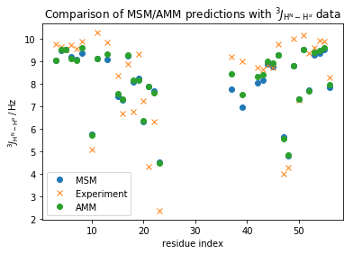
plt.plot(np.array(md_phi_rindex)[idx_md], M_gb3.stationary_distribution.dot(_E[:,idx_md]),'o',label='MSM')
plt.plot(expljc[idx_expl,0], expljc[idx_expl,1],'x', label='Experiment')
plt.plot(expljc[idx_expl,0], amm_gb3.mhat,'o', label='AMM')

plt.xlabel('residue index')
plt.ylabel(r'$^3J_{\mathrm{H}^{\mathrm{N}}-\mathrm{H}^{\alpha}}\, / \, \mathrm{Hz}$')
plt.title(r'Comparison of MSM/AMM predictions with $^3J_{\mathrm{H}^{\mathrm{N}}-\mathrm{H}^{\alpha}}$ data')

plt.legend()

<matplotlib.legend.Legend at 0x125883898>

print("RMS error MSM: {:.3f}".format(np.std(M_gb3.stationary_distribution.dot(_E[:,idx_md])-expljc[idx_expl,1])))
print("RMS error AMM: {:.3f}".format(np.std(amm_gb3.mhat-expljc[idx_expl,1])))

RMS error MSM: 1.103
RMS error AMM: 1.048

This improved the overall fit a bit, but some individual data-points improve a lot - Let us now coarse-grain the model into 2 meta-stable states using PCCA, to better understand what changes including the experimental data result in:

M_gb3.pcca(2)
amm_gb3.pcca(2)

<pyemma.msm.models.pcca.PCCA at 0x12412c710>

colors = ['orange', 'magenta']

fig,ax=plt.subplots(ncols=2,figsize=(8,4))

pe.plots.scatter_contour(cx, cy, -np.log(M_gb3.stationary_distribution), cmap='viridis',ax=ax[0])
pe.plots.scatter_contour(cx, cy, -np.log(amm_gb3.stationary_distribution), cmap='viridis',ax=ax[1])

for i, st in enumerate(M_gb3.metastable_sets):
    ax[0].scatter(cx[st], cy[st], c = colors[i], s = 5)
for i, st in enumerate(amm_gb3.metastable_sets):
    ax[1].scatter(cx[st], cy[st], c = colors[i], s = 5)

ax[0].set_title('GB3 MSM')
ax[1].set_title('GB3 AMM (scalar couplings)')
fig.tight_layout(pad=2.5)

fig.suptitle(r'$-\log{\pi_i}$ plots', fontsize=16)

<matplotlib.text.Text at 0x11e7377f0>

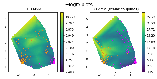
We show minus log probabilities of the GB3 MSM and the GB3 AMM, and show the different meta-stable assignments using orange and magenta colors. Note how the meta-stable state assignments are slightly different in the two model in low-probability regions.

Some regions of conformational space are substantially downweighed in the AMM, in particular in the orange meta-stable configuration. Let’s compare the coarse-grained stationary distributions to better quantify these differences:

fig, ax=plt.subplots(figsize=(4,4))
xticks = []
for i, st in enumerate(M_gb3.metastable_sets):
    ax.bar(i/2.-0.11, M_gb3.stationary_distribution[st].sum(), color = colors[i], width = .2)
    ax.text(i/2.-0.11-0.055, M_gb3.stationary_distribution[st].sum()+0.01, "{:.3f}".format(M_gb3.stationary_distribution[st].sum()))
    xticks.append(i/2.-0.11)

for i, st in enumerate(amm_gb3.metastable_sets):
    ax.bar(i/2.+0.11, amm_gb3.stationary_distribution[st].sum(), color = colors[i], width = .2)
    ax.text(i/2.+0.11/2., amm_gb3.stationary_distribution[st].sum()+0.01, "{:.3f}".format(amm_gb3.stationary_distribution[st].sum()))
    xticks.append(i/2.+0.11)
ax.set_xticks(xticks)
ax.set_ylim((0.,1.05))
ax.set_xticklabels([ 'MSM','MSM', 'AMM', 'AMM'], rotation = 45)
ax.set_ylabel('probability of meta-stable state')

<matplotlib.text.Text at 0x11f0aa4a8>

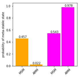
We see a strong repopulation towards the magenta state in the AMM compared to the MSM.

Finally, let us inspect the slowest time-scale of the AMM vs the MSM:

print("Slowest MSM time-scale is {:.3f} microseconds.".format(M_gb3.timescales(k = 1)[0]*time_step_ps/1e6))
print("Slowest AMM time-scale is {:.3f} microseconds.".format(amm_gb3.timescales(k = 1)[0]*time_step_ps/1e6))

Slowest MSM time-scale is 1.367 microseconds.
Slowest AMM time-scale is 2.582 microseconds.

In this case we see a slow-down of the slowest time-scale. But note this value is very sensitive to numerical fluctuations in the estimation algorithm such as number of cluster-centers as we have very little simulation data in this example. Consequently, caution must be taken before making inferences about changes in time-scales with small data-sets like this. Generally we recommend repeating the estimation with multiple independent discretizations to test the robustness of these values. The meta-stable state distribution will also fluctuate as we change the number of clusters but this result is generally more robust.

Validations and sanity checks

To finish off, we will inspect our estimated AMM to ensure everything makes sense.

An interesting thing to inspect first is the Lagrange multipliers \(\lambda_i\), which compensate for the systematic errors between the simulation and experimental ensembles.

fig,ax=plt.subplots(ncols=3,figsize=(12,4))

ax[0].plot(expljc[idx_expl,0], amm_gb3.lagrange, 'o')
ax[0].set_xlabel('residue index')
ax[0].set_ylabel(r'$\lambda_i$')

ax[1].hist(amm_gb3.lagrange)
ax[1].set_xlabel(r'$\lambda_i$')
ax[1].set_ylabel(r'count $\lambda_i$')

ax[2].scatter(amm_gb3.lagrange, amm_gb3.m-M_gb3.stationary_distribution.dot(_E[:,idx_md]) )
ax[2].set_xlabel(r'$\lambda_i$')
ax[2].set_ylabel(r'MSM prediction error')

fig.tight_layout()

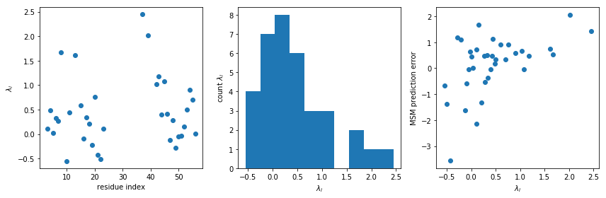
We see many of the Lagrange multipliers cluster around zero, which is good news for the forcefield as it illustratess that a substantial fraction of the observables are fairly well described by the unbiased simulation. However, a few larger values are also seen – this can mean three different things: * the forcefield does not describe this observable well, * we have under-estimated the uncertainty of these observations * the experimental values are not assigned to the right molecular feature.

The latter of these points can be due either to mislabeling in either the computational analysis or on the experimental side.

Note, the weak correlation between the MSM prediction error of our AMM lagrange multipliers is visible, which is naively expected.

Next, we look at population weighed variances of our experimental observable in the MSMs and AMMs,

\[\sigma_i^2(\pi) = \sum_j \pi_j(E_{ji}-e_i)^2\]

where $ e_i = \sum_j \pij E{ji}$ (the expectation of observable \(i\)), \(\pi\) is the stationary vector of the AMM or MSM and the \(E\)-matrix is as defined above.

fig, ax=plt.subplots(ncols=1,figsize=(6,4))

msm_obs_var = M_gb3.stationary_distribution.dot((amm_gb3.E_active- M_gb3.stationary_distribution.dot(amm_gb3.E_active))**2. )
amm_obs_var = amm_gb3.stationary_distribution.dot((amm_gb3.E_active-amm_gb3.mhat)**2.)

ax.semilogy(expljc[idx_expl,0], amm_obs_var, 'o', label="AMM")
ax.semilogy(expljc[idx_expl,0], msm_obs_var, 'x', label="MSM")
ax.set_xlabel('residue index')
ax.set_ylabel(r'$\mathrm{var} (J)\; \; / \; \; \mathrm{Hz}^2$')
ax.legend()
fig.tight_layout()

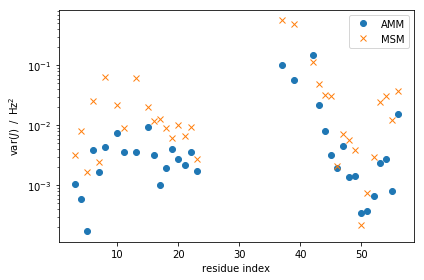
We generally expect these variances to decrease as we are enforcing additional information about these quantities. Indeed, we see most of these decreasing dramatically, and a few remaining more or less unchanged. Note the log-scale on the y-axis.

Cross-validation with other experimental data

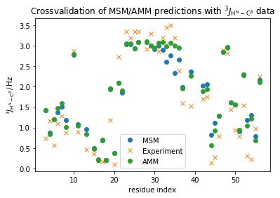
Finally, we cross-validate the AMM using another set of scalar-couplings which are also sensitive to the backbone \(\phi\) angle but is measured through the dihedral between the planes defined by the vectors (\(H^N-N\), \(N-C^{\alpha}\)) the (\(C^{\alpha}-C^{\beta}\),\(C^{\alpha}-N\)).

For this we can reuse alot of our featurization from above - but need a new set of Karplus parameters:

A2_ = 3.693
B2_ = -0.514
C2_ = 0.043

# Load data
expljc2 = np.loadtxt('gb3_data/HN_CB_JC.dat')

#Compute scalar-couplings
Phi_all = np.vstack(phis_)+np.pi/3 # correct the phase
cosPhi_all = np.cos(Phi_all)
cossqPhi_all = cosPhi_all*cosPhi_all
JC_all = A2_*cossqPhi_all+B2_*cosPhi_all+C2_

#Find intersection in set of computable and measured scalar couplings.
a=[int(i) for i in set(md_phi_rindex).intersection(expljc2[:,0])]
idx_expl = [np.where(expljc2[:,0]==i)[0][0] for i in a]
idx_md = [np.where(np.array(md_phi_rindex)==i)[0][0] for i in a]

# Compute E-matrix
dta = np.concatenate(dtrajs)
all_markov_states = set(dta)
_E = np.zeros((len(all_markov_states), JC_all.shape[1]))
for i, s in enumerate(all_markov_states):
    _E[i, :] = JC_all[np.where(dta == s)].mean(axis = 0)

plt.plot(np.array(md_phi_rindex)[idx_md], M_gb3.stationary_distribution.dot(_E[:,idx_md]),'o',label='MSM')
plt.plot(expljc2[idx_expl,0], expljc2[idx_expl,1],'x', label='Experiment')
plt.plot(np.array(md_phi_rindex)[idx_md], amm_gb3.stationary_distribution.dot(_E[:,idx_md]),'o',label='AMM')

plt.xlabel('residue index')
plt.ylabel(r'$^3J_{\mathrm{H}^{\mathrm{N}}-\mathrm{C}^{\beta}}\, / \, \mathrm{Hz}$')
plt.title(r'Crossvalidation of MSM/AMM predictions with $^3J_{\mathrm{H}^{\mathrm{N}}-\mathrm{C}^{\beta}}$ data')

plt.legend()

<matplotlib.legend.Legend at 0x124cb1f28>

print("RMS MSM: {:.3f}".format(np.std(M_gb3.stationary_distribution.dot(_E[:,idx_md])-expljc2[idx_expl,1])))
print("RMS AMM: {:.3f}".format(np.std(amm_gb3.stationary_distribution.dot(_E[:,idx_md])-expljc2[idx_expl,1])))

RMS MSM: 0.502
RMS AMM: 0.443

We observe an ever so slight improvement in the agreement with these complementary experimental data which suggests that our AMM is an overall more accurate model compared to the MSM.

Cross-validating with relaxation-dispersion data and other dynamic observables

Is covered in this notebook and here.

Double-checking AMM estimation convergence

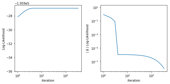
Sometimes it is instructutive to inspect model log-likelihood as a function of iteration, along with its absolute \(\Delta\). Current default values for convergence is when \(\Delta\) is less than \(10^{-8}\).

fig,ax=plt.subplots(ncols=2,figsize=(8,4))

ax[0].semilogx(amm_gb3._lls, '-')
ax[0].set_xlabel('iteration')
ax[0].set_ylabel(r'Log-Likelihood')

ax[1].loglog(np.abs(np.diff(amm_gb3._lls[:])))
ax[1].set_xlabel(r'iteration')
ax[1].set_ylabel(r'$\mid\Delta\mid$Log-Likelihood')

fig.tight_layout()